
In the generalized linear models tutorial, we learned about various GLM’s like linear regression, logistic regression, etc.. In this tutorial of the TechVidvan’s R tutorial series, we are going to look at linear regression in R in detail. We will learn what is R linear regression and how to implement it in R. We will look at the least square estimation method and will also learn how to check the accuracy of the model.
So, without any further ado, let’s get started!

Linear Regression in R
Linear regression in R is a method used to predict the value of a variable using the value(s) of one or more input predictor variables. The goal of linear regression is to establish a linear relationship between the desired output variable and the input predictors.
To model a continuous variable Y as a function of one or more input predictor variables Xi, so that the function can be used to predict the value of Y when only the values of Xi are known. The general form of such a linear relationship is:
Y=?0+?1 X
Here, ?0 is the intercept
and ?1 is the slope.
Types of Linear Regression in R
There are two types of R linear regression:
- Simple Linear Regression
- Multiple Linear Regression
Let’s take a look at these one-by-one.
Simple Linear Regression in R
Simple linear regression is aimed at finding a linear relationship between two continuous variables. It is important to note that the relationship is statistical in nature and not deterministic.
A deterministic relationship is one where the value of one variable can be found accurately by using the value of the other variable. An example of a deterministic relationship is the one between kilometers and miles. Using the kilometer value, we can accurately find the distance in miles. A statistical relationship is not accurate and always has a prediction error. For example, given enough data, we can find a relationship between the height and the weight of a person, but there will always be a margin of error and exceptional cases will exist.
The idea behind simple linear regression is to find a line that best fits the given values of both variables. This line can then help us find the values of the dependent variable when they are missing.
Let us study this with the help of an example. We have a dataset consisting of the heights and weights of 500 people. Our aim here is to build a linear regression model that formulates the relationship between height and weight, such that when we give height(Y) as input to the model it may give weight(X) in return to us with minimum margin or error.
Y=b0+b1X
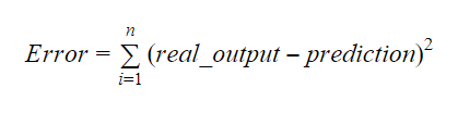
The values of b0 and b1 should be chosen so that they minimize the margin of error. The error metric can be used to measure the accuracy of the model.
We can calculate the slope or the co-efficient as:
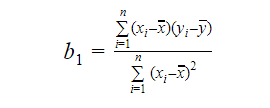
The value of b1 gives us insight into the nature of the relationship between the dependent and the independent variables.
- If b1 > 0, then the variables have a positive relationship i.e. increase in x will result in an increase in y.
- If b1 < 0, then the variables have a negative relationship i.e. increase in x will result in a decrease in y.
The value of b0 or intercept can be calculated as follows:

If the model does not include x=0, then the prediction is meaningless without b1. For the model to only have b0 and not b1 in it at any point, the value of x has to be 0 at that point. In cases such as height, x cannot be 0 and a person’s height cannot be 0. Therefore, such a model is meaningless with only b0.
If the b0 term is missing then the model will pass through the origin, which will mean that the prediction and the regression coefficient(slope) will be biased.
Multiple Linear Regression in R
Multiple linear regression is an extension of simple linear regression. In multiple linear regression, we aim to create a linear model that can predict the value of the target variable using the values of multiple predictor variables. The general form of such a function is as follows:
Y=b0+b1X1+b2X2+…+bnXn
Assessing the Accuracy of the Model
There are various methods to assess the quality and accuracy of the model. Let’s take a look at some of these methods one at a time.
1. R-Squared
The real information in data is the variance conveyed in it. R-squared tells us the proportion of variation in the target variable (y) explained by the model. We can find the R-squared measure of a model using the following formula:
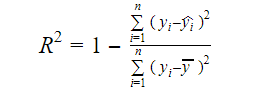
Where,
- yi is the fitted value of y for observation i
- y is the mean of Y.
A lower value of R-squared signifies a lower accuracy of the model. However, the R-squared measure is not necessarily a final deciding factor.
2. Adjusted R-Squared
As the number of variables increases in the model, the R-squared value increases as well. This also causes errors in the variation explained by the newly added variables. Therefore, we adjust the formula for R square for multiple variables.
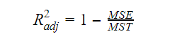

And MST stands for Mean Standard Total which is given by:
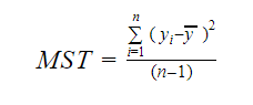
Where, n is the number of observations and q is the number of coefficients.
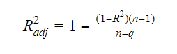
The relationship between R-squared and adjusted R-squared is:
3. Standard Error and F-Statistic
The standard error and the F-statistic are both measures of the quality of the fit of a model. The formulae for standard error and F-statistic are:
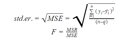
Where MSR stands for Mean Square Regression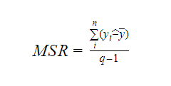
4. AIC and BIC
Akaike’s Information Criterion and Bayesian Information Criterion are measures of the quality of the fit of statistical models. They can also be used as criteria for the selection of a model.
AIC=(-2)*ln(L)+2*k
BIC=(-2)*ln(L)+k*ln(n)
Where,
- L is the likelihood function,
- k is the number of model parameters,
- n is the sample size.
lm function in R
The lm() function of R fits linear models. It can carry out regression, and analysis of variance and covariance. The syntax of the lm function is as follows:
lm(formula, data, subset, weights, na.action,
method = "qr", model = TRUE, x = FALSE, y = FALSE, qr = TRUE,
singular.ok = TRUE, offset, …)
Where,
- formula is an object of class “formula” and is a symbolic representation of the model to fit,
- data is the data frame or list that contains the variables in the formula(data is an optional argument. If it is missing, the function picks up the variables from the environment),
- subset is an optional vector containing a subset of observations that are to be used in the fitting process,
- weights is an optional vector that specifies the weights to be used in the fitting process,
- na.action is a function that shows what should happen when NA’s are encountered in the data,
- method signifies the method for fitting the model,
- model, x, y, and qr are logicals that control whether corresponding values should be returned with the output or not. These values are:
- model: the model frame
- x: the model matrix
- y: the response
- qr: the qr decomposition
- singular.ok is a logical that control whether singular fits are allowed or not,
- offset is a priorly known predictor that should be used in the model,
- . . . are additional arguments to be passed to the lower level regression functions.
Practical Example of Linear Regression in R
That is enough theory for now. Let us take a look at how to implement all this. We are going to fit a linear model using linear regression in R with the help of the lm() function. We will also check the quality of fit of the model afterward. Let’s use the cars dataset which is provided by default in the base R package.
1. Let us start with a graphical analysis of the dataset to get more familiar with it. To do that we will draw a scatter plot and check what it tells us about the data.
We can use scatter.smooth() function to create a scatter plot for the dataset.
scatter.smooth(x=cars$speed,y=cars$dist,main="TechVidvan Dist ~ Speed")
Output
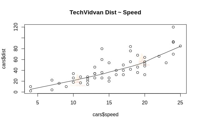
The scatter plot shows us a positive correlation between distance and speed. It suggests a linearly increasing relationship between the two variables. This makes the data suitable for linear regression as a linear relationship is a basic assumption for fitting a linear model on data.
2. Now that we have verified that linear regression is suitable for the data, we can use the lm() function to fit a linear model to it.
Linear_model <- lm(dist~speed,data=cars)
print(Linear_model)
Output
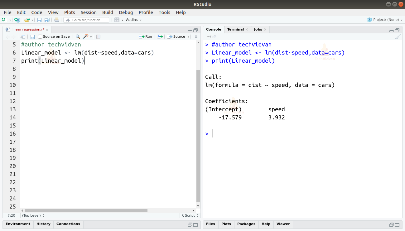
The output of the lm() function shows us the intercept and the coefficient of speed. Thus defining the linear relationship between distance and speed as:
Distance=Intercept+coefficient*speed
Distance=-17.579+3.932*speed
3. Now that we have fitted a model let us check the quality or goodness of the fit. Let us start by checking the summary of the linear model by using the summary() function.
summary(Linear_model)
Output
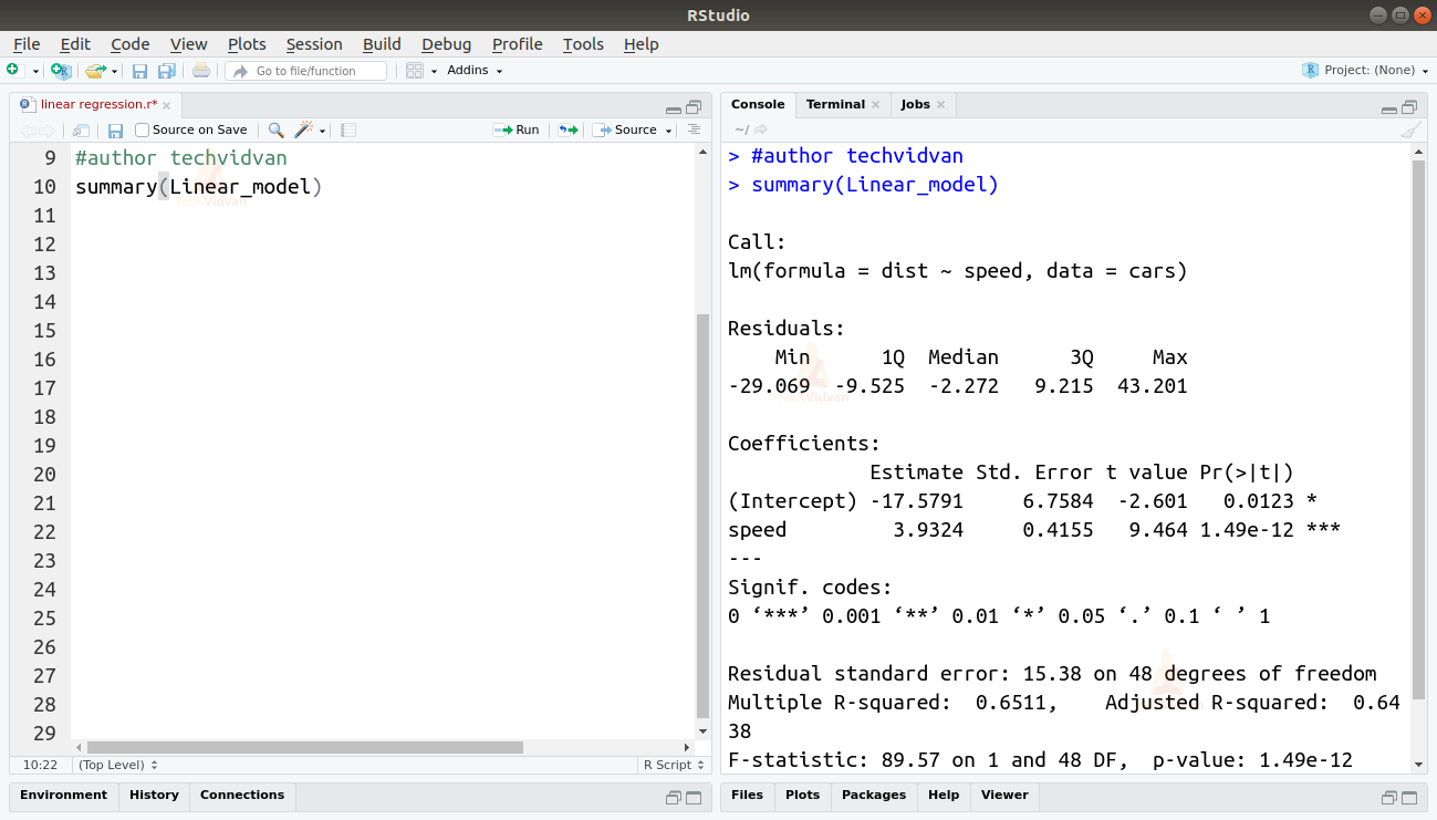
The summary() function gives us a few important measures to help diagnose the fit of the model. The p-value is an important measure of the goodness of the fit of a model. A model is said to not be fit if the p-value is more than a pre-determined statistical significance level which is ideally 0.05.
The summary also provides us with the t-value. The more the t-value the better fit the model is.
We can also find the AIC and BIC by using the AIC() and the BIC() functions.
AIC(Linear_model)
BIC(Linear_model)
Output
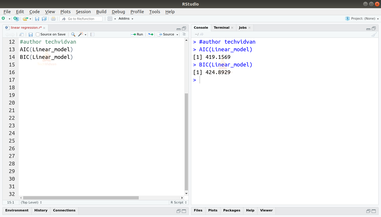
The model which results in the lowest AIC and BIC scores is the most preferred.
Summary
In this chapter of the TechVidvan’s R tutorial series, we learned about linear regression. We learned about simple linear regression and multiple linear regression. Then we studied various measures to assess the quality or accuracy of the model, like the R2, adjusted R2, standard error, F-statistics, AIC, and BIC. We then learned how to implement linear regression in R. We then checked the quality of the fit of the model in R.
Do share your rating on Google if you liked the Linear Regression tutorial.