
In the previous R tutorial, we learned about linear regression and how to implement it in R. With this chapter of TechVidvan’s R tutorial series, we are going to study non-linear regression in R. We will learn what R non-linear regression is? We will also learn the various kinds of non-linear regression models in R. Finally, we will look at how to implement non-linear regression in R.
Non-Linear Regression in R
R Non-linear regression is a regression analysis method to predict a target variable using a non-linear function consisting of parameters and one or more independent variables. Non-linear regression is often more accurate as it learns the variations and dependencies of the data.
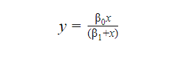
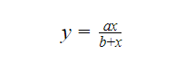
Non-linear functions can be very confusing for beginners. For example, let’s check out the following function.
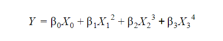
Now, you might think that this equation can represent a non-linear model, but that is not true. The above equation is, in fact, a linear regression equation. The easiest way to identify a linear regression function in R is to look at the parameters. The above equation is linear in the parameters, and hence, is a linear regression function. The basic format of a linear regression equation is as follows:
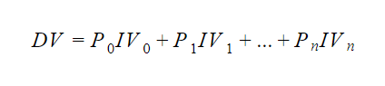
Where
- DV is the dependent variable,
- P0,P1,…Pn are the parameters,
- IV0,IV1, . . . IVn are independent variables.
These independent variables can be logarithmic, exponential, squared, cubic, quadratic, or raised to any power. As long as a regression function fits the format, it is a linear regression function. A model may call as non-linear regression model if its function does not fit the linear regression function format.
Here are a few examples of non-linear equations:
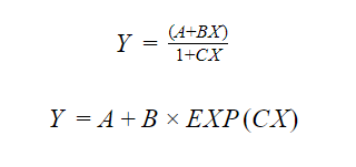
There are also certain non-linear functions that can modify with algebra to mimic the linear format. For example,
This equation can be rewritten as:
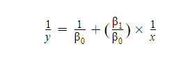
Such non-linear functions that can be rewritten as linear functions are said to be intrinsically linear.
Maximum Likelihood Estimation
Maximum likelihood estimation is a method for estimating the values of the parameters to best fit the chosen model. It provides estimated values for the parameters of the model equation that maximize the likelihood of the predicted values matching the actual data.
MLE treats finding model parameters as an optimization problem. It seeks a set of parameters that result in the best fit of the joint probability of the given data.
Examples of Non-Linear Regression Models
1. Logistic regression model
Logistic regression is a type of non-linear regression model. It is most commonly used when the target variable or the dependent variable is categorical. For example, whether a tumor is malignant or benign, or whether an email is useful or spam.
Linear regression models work better with continuous variables. When working with categorical variables, outputs as continuous values may result in incorrect classifications.
There are three kinds of logistic regression models:
- Binary logistic models
These types of models only have two possible outcomes. For example, a tumor being benign or malignant.
- Multinomial logistic models
These types of models have three or more possible outcomes with no order of preference or ranking. For example, what types of beverages are more preferred(smoothie, milkshake, juice, tea, coffee, etc.)
- Ordinal logistic models
These types of models have three or more possible outcomes and these outcomes have an order of preference. For example, Movie ratings from 1 to 5 stars.
2. Michaelis-Menten Regression model
Michaelis-Menten Kinetics model is the most popular kinetics model, used for modeling enzyme kinetics in biochemistry. It is named after a biochemist from Germany named Leonor Michaelis and a Physician from Canada named Maud Menten. The model describes the rate of enzymatic reactions by relating the reaction rate to the concentration of a substrate. The equation looks something like this: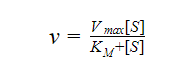
- Vmax is the maximum rate achieved by the system,
- KM is the Michaelis coefficient,
- S is the concentration of the substrate,
- v is the rate of the enzymatic reaction.
3. Generalized Additive Models
Generalized additive models fit non-parametric curves to given data without needing a specific mathematical model to describe the nonlinear relationship between the variables. They are very useful as they allow us to identify the relationships between dependent and independent variables without requiring a particular parametric form. The gam() function in R can be used to fit data to curves using the generalized additive models in R.
Changing Non-Linear Models Into Linear Models
Sometimes non-linear models are converted into linear models and fitted to curves using certain techniques. This is done with the aim of simplifying the process of fitting the data to the curve as it is easier to fit a linear model than a non-linear model.
Let us take a look at this using an example. The following equation clearly represents a non-linear regression model.
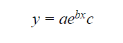
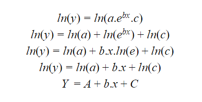
Where
- Y is ln(y),
- A = ln(A),
- C = ln(c).
As we can see, this equation has now taken the shape and form of a linear regression equation and will be much easier to fit to a curve.
nls Function in R
The nls() function in R is very useful for fitting non-linear models. NLS stands for Nonlinear Least Square. The nls() function fits a non-linear model using the least square estimation method. The syntax of the nls function is as follows:
nls(formula, data, start, control, algorithm, trace, subset, weights, na.action, model, lower, upper, . . .)
Where
- formula is a non-linear formula consisting of variables and parameters,
- data is the input dataset,
- start is a named list or numeric vector of starting variables,
- control is an optional list of control setting,
- algorithm is a string that specifies which algorithm to use,
- trace is a logical variable that indicates whether a trace of the progress of the iterations should be printed or not,
- subset is an option vector consisting of observations for the fitting process,
- weights is an optional numeric vector of fixed weights,
- na.action that indicates what the function should do when the data contains NS values,
- model is a logical which indicates that the model frame should be returned as the output when it is set to TRUE,
- lower and upper are vectors of the lower and upper bounds of the data.
Example of Non-Linear Regression in R
As a practical demonstration of non-linear regression in R. Let us implement the Michaelis Menten model in R.
As we saw in the formula above, the model we are going to implement has two variables and two parameters.

We can rewrite the above equation as:
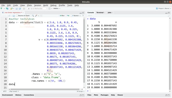
1. Let us get a dataset to work with.
data <- structure(list(S = c(3.6, 1.8, 0.9, 0.45,
                           0.225, 0.1125, 3.6,
                           1.8, 0.9, 0.45, 0.225,
                           0.1125, 3.6, 1.8, 0.9,
                           0.45, 0.225, 0.1125, 0),
                     v = c(0.004407692, 0.004192308,
                           0.003553846, 0.002576923,
                           0.001661538, 0.001064286,
                           0.004835714, 0.004671429,
                           0.0039, 0.002857143,
                           0.00175, 0.001057143,
                           0.004907143, 0.004521429,
                           0.00375, 0.002764286,
                           0.001857143, 0.001121429,
                           0)),
                .Names = c("S", "v"),
                class = "data.frame",
                row.names = c(NA, -19L))
data
Output
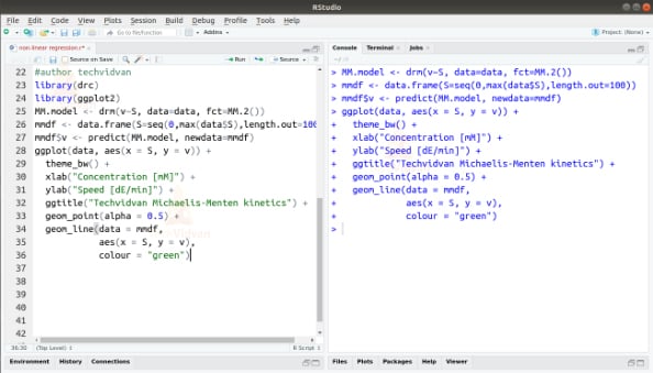
2. Once we have our data, we can use the drc package to fit it to a curve. We can also use the ggplot2 package to plot the data as well.
library(drc)
library(ggplot2)
MM.model <- drm(v~S, data=data, fct=MM.2())
mmdf <- data.frame(S=seq(0,max(data$S),length.out=100))
mmdf$v <- predict(MM.model, newdata=mmdf)
ggplot(data, aes(x = S, y = v)) +
theme_bw() +
xlab("Concentration [mM]") +
ylab("Speed [dE/min]") +
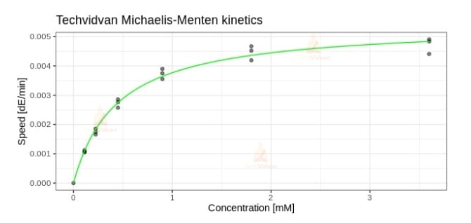
ggtitle("Techvidvan Michaelis-Menten kinetics") +
geom_point(alpha = 0.5) +
geom_line(data = mmdf,
aes(x = S, y = v),
colour = "green")
Output
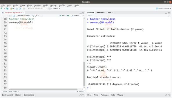
3. We can see the summary of the model by using the summary() function.
summary(MM.model)
Output
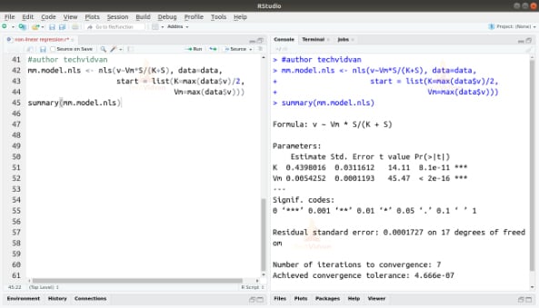
4. We can also perform regression and plot it using the nls() function. Let’s give that a try.
mm.model.nls <- nls(v~Vm*S/(K+S), data=data,
                    start = list(K=max(data$v)/2,
                                 Vm=max(data$v)))
summary(mm.model.nls)
Output
Summary
In this chapter of the TechVidvan’s R tutorial series, we learned about non-linear regression in R. We studied what non-linear regression is and what different types of regression models are considered to be non-linear. Then we looked at the maximum likelihood estimation method. We further learned about logistic regression, Michaelis-Menten regression, and generalized additive models. Finally, We also studied how to transform non-linear models into linear models and why we may want to do so. Finally, we learned how to implement a non-linear regression model in R.
Do not forget to share your Google rating if you liked the article.