Vehicle Counting, Classification & Detection using OpenCV & Python
Today, we’re going to build an advanced vehicle detection and classification project using OpenCV. We’ll use the YOLOv3 model with OpenCV-python. Open-CV is a real-time computer vision library of Python. We can use YOLO directly with OpenCV.
What is YOLO?
YOLO stands for You Only Look Once. It is a real-time object recognition algorithm. It can classify and localize multiple objects in a single frame. YOLO is a very fast and accurate algorithm for its simpler network architecture.
How does YOLO work?
YOLO works using mainly these techniques.
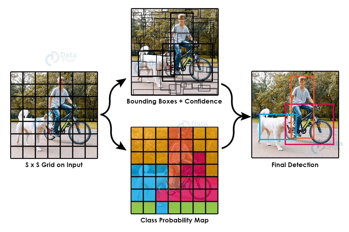
1. Residual Blocks – Basically, it divides an image into NxN grids.
2. Bounding Box regression – Each grid cell is sent to the model. Then YOLO determines the probability of the cell contains a certain class and the class with the maximum probability is chosen.
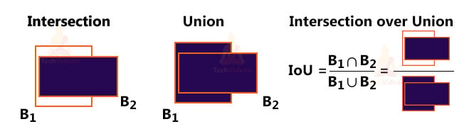
3. Intersection Over Union (IOU) – IOU is a metric that evaluates intersection between the predicted bounding box and the ground truth bounding box. A Non-max suppression technique is applied to eliminate the bounding boxes that are very close by performing the IoU with the one having the highest class probability among them.
Here is the combination of these 3 techniques.
YOLO Architecture :
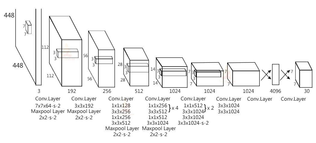
- The YOLO network has 24 convolutional layers followed by 2 fully connected layers. The convolutional layers are pre-trained on the ImageNet classification task at half the resolution (224 × 224 input image) and then double the resolution for detection.
- The layers Alternating 1 × 1 reduction layer and 3×3 convolutional layer to reduce the feature space from preceding layers.
- The last 4 layers are added to train the network for object detection.
- The last layer predicts the object class probability and the bounding box probability.
We’ll use OpenCV’s DNN module to work with YOLO directly. DNN means Deep Neural Network. OpenCV has a built-in function to perform DNN algorithms.
OpenCV Vehicle Detection and Classification Project
In this project, we’ll detect and classify cars, HMV ( Heavy Motor Vehicle) , LMV (Light Motor Vehicle) on the road, and count the number of vehicles traveling through a road. And the data will be stored to analyze different vehicles that travel through the road.
We’ll create two programs to do this project. The first one will be the tracker for vehicle detection using OpenCV that keeps track of each and every detected vehicle on the road and the 2nd one will be the main detection program.
Prerequisites for Vehicle Detection and Classification Project using OpenCV:
1. Python – 3.x (We used python 3.8.8 in this project)
2. OpenCV – 4.4.0
- It is strongly recommended to run DNN models on GPU.
- You can install OpenCV via “pip install opencv-python opencv_contrib-python”.
3. Numpy – 1.20.3
4. YOLOv3 Pre-trained model weights and Config Files.
Download Vehicle Detection & Classification Python OpenCV Code
Please download the source code of opencv vehicle detection & classification: Vehicle Detection and Classification OpenCV Code
Tracker:
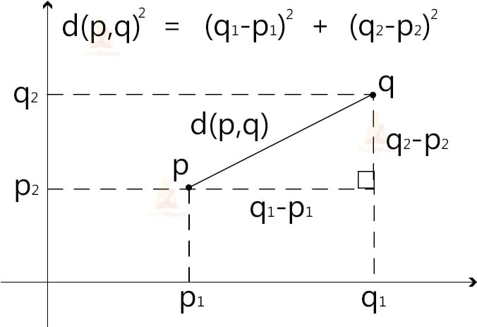
The tracker basically uses the Euclidean_distance concept to keep track of an object. It calculates the difference between two center points of an object in the current frame vs the previous frame, and if the distance is less than the threshold distance then it confirms that the object is the same object of the previous frame.
Import math

      # Get center point of new object
      for rect in objects_rect:
          x, y, w, h, index = rect
          cx = (x + x + w) // 2
          cy = (y + y + h) // 2

          # Find out if that object was detected already
          same_object_detected = False
          for id, pt in self.center_points.items():
              dist = math.hypot(cx - pt[0], cy - pt[1])

              if dist < 25:
                  self.center_points[id] = (cx, cy)
                  # print(self.center_points)
                  objects_bbs_ids.append([x, y, w, h, id, index])
                  same_object_detected = True
                  break
- The math.hypot() method returns the Euclidean distance.
- Here we check if the distance is less than 25 then the object is the same object of the previous frame.
Vehicle Counter:
Steps for Vehicle Detection and Classification using OpenCV:
1. Import necessary packages and Initialize the network.
2. Read frames from a video file.
3. Pre-process the frame and run the detection.
4. Post-process the output data.
5. Track and count all vehicles on the road
6. Save the final data to a CSV file.
Step 1 – Import necessary packages and Initialize the network:
import cv2
import csv
import collections
import numpy as np
from tracker import *

# Initialize Tracker
tracker = EuclideanDistTracker()

# Detection confidence threshold
confThreshold =0.1
nmsThreshold= 0.2
- First, we import all the necessary packages we need for the project.
- Then, we initialize the EuclideanDistTracker() object from the tracker program we’ve created before and set the object as “tracker”.
- confThreshold and nmsThreshold are minimum confidence score threshold for detection and Non-Max suppression threshold respectively.
  # Middle cross line position
middle_line_position = 225
up_line_position = middle_line_position - 15
down_line_position = middle_line_position + 15
- These line positions are the crossing line positions that will be used to count vehicles.
Note: Modify middle_line_position according to your need.
# Store Coco Names in a list

classesFile = "coco.names"
classNames = open(classesFile).read().strip().split('\n')
print(classNames)
print(len(classNames))
- YOLOv3 is trained on the COCO dataset, so we read the file that contains all the class names and store the names in a list.
- The COCO dataset contains 80 different classes.
- We need to detect only cars, motorbikes, buses, and trucks for this project, that’s why the required_class_index contains the index of those classes from the coco dataset.
Output-
## Model Files
modelConfiguration = 'yolov3-320.cfg'
modelWeights = 'yolov3-320.weights'

# configure the network model
net = cv2.dnn.readNetFromDarknet(modelConfiguration, modelWeights)

# Configure the network backend

net.setPreferableBackend(cv2.dnn.DNN_BACKEND_CUDA)
net.setPreferableTarget(cv2.dnn.DNN_TARGET_CUDA)

# Define random colour for each class
np.random.seed(42)
colors = np.random.randint(0, 255, size=(len(classNames), 3), dtype='uint8')
- Configure the network using cv2.dnn.readNetFromDarknet() function.
- Here we’re using GPU, that’s why we set “net.setPreferableBackend” as DNN_BACKEND_CUDA and net.setPreferableTarget as DNN_TARGET_CUDA.
- If you’re using GPU, set the DNN backend as CUDA and if you’re using CPU then you can comment out those lines.
- Using np.random.randint() function we generate a random color for each class in our dataset. We’ll use these colors to draw the rectangles around the objects.
- random.seed() function saves the state of a random function so that it can generate some random number on every execution, even if it will generate the same random numbers in other machines too.
Step 2 – Read frames from a Video file:
# Initialize the videocapture object
cap = cv2.VideoCapture('video.mp4')
def realTime():
while True:
success, img = cap.read()
img = cv2.resize(img,(0,0),None,0.5,0.5)
ih, iw, channels = img.shape
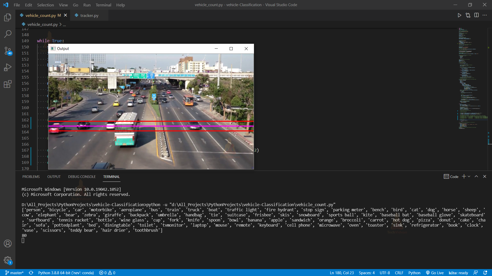
# Draw the crossing lines
cv2.line(img, (0, middle_line_position), (iw, middle_line_position),
(255, 0, 255), 1)
cv2.line(img, (0, up_line_position), (iw, up_line_position), (0, 0, 255), 1)
cv2.line(img, (0, down_line_position), (iw, down_line_position), (0, 0, 255), 1)
# Show the frames
cv2.imshow('Output', img)
if __name__ == '__main__':
realTime()
- Read the video file through the videoCapture object and set the object as cap.
- cap.read() reads each frame from the capture object.
- Using cv2.reshape() we reduced our frame by 50 percent.
- Then using the cv2.line() function we draw the crossing lines in the frame.
- And finally, we used cv2.imshow() function to show the output image.
Step 3 – Pre-process the frame and run the detection:
input_size = 320

   blob = cv2.dnn.blobFromImage(img, 1 / 255, (input_size, input_size), [0, 0, 0], 1, crop=False)

   # Set the input of the network
   net.setInput(blob)
   layersNames = net.getLayerNames()
   outputNames = [(layersNames[i[0] - 1]) for i in net.getUnconnectedOutLayers()]
   # Feed data to the network
   outputs = net.forward(outputNames)

   # Find the objects from the network output
   postProcess(outputs,img)
- Our version of YOLO takes 320×320 image objects as input. The input to the network is a blob object. The function dnn.blobFromImage() takes an image as input and returns a resized and normalized blob object.
- The net.forward() is used to feed the image to the network. And it returns an output.
- And finally, we call our custom postProcess() function to post-process the output.
Step 4 – Post-process the output data:
The network forward output contains 3 outputs. Each output object is a vector of length 85.
- 4x the bounding box (centerX, centerY, width, height)
- 1x box confidence
- 80x class confidence
So, let’s define our post-processing function.
detected_classNames = []
def postProcess(outputs,img):
   global detected_classNames
   height, width = img.shape[:2]
    boxes = []
    classIds = []
    confidence_scores = []
    detection = []
    for output in outputs:
        for det in output:
            scores = det[5:]
            classId = np.argmax(scores)
            confidence = scores[classId]
            if classId in required_class_index:
                if confidence > confThreshold:
                    # print(classId)
                    w,h = int(det[2]*width) , int(det[3]*height)
                    x,y = int((det[0]*width)-w/2) , int((det[1]*height)-h/2)
                    boxes.append([x,y,w,h])
                    classIds.append(classId)
                    confidence_scores.append(float(confidence))
- First, we defined an empty list ‘detected_classNames’ where we’ll store all the detected classes in a frame.
- Using two for loops we iterate through each vector of each output and collect confidence score and classId index.
- After that, we check if the class confidence score is greater than our defined confThreshold. Then we collect the information about the class and store the box coordinate points, class-Id, and Confidence score in three separate lists.
→Non-Max Suppression:-
YOLO sometimes gives multiple bounding boxes for a single object, so we have to reduce the number of detection boxes and have to take the best detection box for each class.
   # Apply Non-Max Suppression
    indices = cv2.dnn.NMSBoxes(boxes, confidence_scores, confThreshold,
nmsThreshold)
    # print(classIds)
    for i in indices.flatten():
        x, y, w, h = boxes[i][0], boxes[i][1], boxes[i][2], boxes[i][3]
        # print(x,y,w,h)

        color = [int(c) for c in colors[classIds[i]]]
        name = classNames[classIds[i]]
        detected_classNames.append(name)


        # Draw classname and confidence score
        cv2.putText(img,f'{name.upper()} {int(confidence_scores[i]*100)}%',
                  (x, y-10), cv2.FONT_HERSHEY_SIMPLEX, 0.5, color, 1)

        # Draw bounding rectangle
        cv2.rectangle(img, (x, y), (x + w, y + h), color, 1)
        detection.append([x, y, w, h, required_class_index.index(classIds[i])])
- Using the NMSBoxes() method we reduce the number of boxes and take only the best detection box for the class.
- cv2.putText draws text in the frame.
- Using cv2.rectangle() we draw the bounding box around the detected object.
Step 5 – Track and count all vehicles on the road:
# Update the tracker for each object
    boxes_ids = tracker.update(detection)
    for box_id in boxes_ids:
        count_vehicle(box_id)
- After getting all the detection, we keep track of those objects using the tracker object. The tracker.update() function keeps track of every detected object and updates the position of the objects.
- Count_vehicle is a custom function that counts the number of vehicles that crossed through the road.
The count_vehicle Function:
# List for store vehicle count information
temp_up_list = []
temp_down_list = []
Create two temporary empty lists to store the vehicles id’s that enter the entry crossing line.
up_list = [0, 0, 0, 0]
down_list = [0, 0, 0, 0]
Up_list and down_list are for counting those 4 vehicle classes in the up route and down route.
# Function for count vehicle
def count_vehicle(box_id):

    x, y, w, h, id, index = box_id

    # Find the center of the rectangle for detection
    center = find_center(x, y, w, h)
    ix, iy = center
The find_center function returns the center point of a rectangle box.
# Find the current position of the vehicle
    if (iy > up_line_position) and (iy < middle_line_position):
        if id not in temp_up_list:
            temp_up_list.append(id)

    elif iy < down_line_position and iy > middle_line_position:
        if id not in temp_down_list:
            temp_down_list.append(id)

    elif iy < up_line_position:
        if id in temp_down_list:
            temp_down_list.remove(id)
            up_list[index] = up_list[index]+1

    elif iy > down_line_position:
        if id in temp_up_list:
            temp_up_list.remove(id)
            down_list[index] = down_list[index] + 1
- In this part, we keep track of each vehicle position and their corresponding Ids.
- First, we check if the object is between the up-crossing line and middle crossing line, then the id of the object is temporality stored in up_list for up route vehicle counting. And we do the opposite for the down route vehicles also.
- And then we check if the object has crossed the down line or not. If the object crossed the down line then the id of the object is counted as an up route vehicle, and we add 1 with the particular type of class counter.
- We need only y coordinate points because we’re counting vehicles on the Y-axis.
# Draw circle in the middle of the rectangle
cv2.circle(img, center, 2, (0, 0, 255), -1)  # end here
# print(up_list, down_list)
Cv2.circle() draws a circle in the frame. In our case, we’re drawing the center point of the car.
  cv2.putText(img, "Up", (110, 20), cv2.FONT_HERSHEY_SIMPLEX, font_size,
font_color, font_thickness)
    cv2.putText(img, "Down", (160, 20), cv2.FONT_HERSHEY_SIMPLEX, font_size,
font_color, font_thickness)
    cv2.putText(img, "Car:        "+str(up_list[0])+"     "+ str(down_list[0]), (20, 40),
cv2.FONT_HERSHEY_SIMPLEX, font_size, font_color, font_thickness)
    cv2.putText(img, "Motorbike:  "+str(up_list[1])+"     "+ str(down_list[1]), (20, 60),
cv2.FONT_HERSHEY_SIMPLEX, font_size, font_color, font_thickness)
    cv2.putText(img, "Bus:        "+str(up_list[2])+"     "+ str(down_list[2]), (20, 80),
cv2.FONT_HERSHEY_SIMPLEX, font_size, font_color, font_thickness)
    cv2.putText(img, "Truck:      "+str(up_list[3])+"     "+ str(down_list[3]), (20, 100),
cv2.FONT_HERSHEY_SIMPLEX, font_size, font_color, font_thickness)
Finally, draw the counts to show the vehicle counting on the frame in real-time.
Vehicle Detection, Counting and Classification Output
Video Source: YouTube
Step 6 – Save the final data to a CSV file:
# Write the vehicle counting information in a file and save it

with open("data.csv", 'w') as f1:
    cwriter = csv.writer(f1)
    cwriter.writerow(['Direction', 'car', 'motorbike', 'bus', 'truck'])
    up_list.insert(0, "Up")
    down_list.insert(0, "Down")
    cwriter.writerow(up_list)
    cwriter.writerow(down_list)
f1.close()
- With the open function, we opened a new file data.csv with write permission only.
- Then we write 3 rows, the first row contains class names and directions, and the 2nd and 3rd row contains up and down route counts respectively.
- The writerow() function writes a row to the file.
Now, let’s do it for a single image:
It is not possible to count vehicles that travel through a road in a particular direction on a static image. Because it is a continuous process. But can classify and count the number of vehicles that are present on the road or an image. And later we can analyze the data.
image_file = 'vehicle classification-image02.png'
def from_static_image(image):
    img = cv2.imread(image)

    blob = cv2.dnn.blobFromImage(img, 1 / 255, (input_size, input_size), [0, 0, 0], 1,
   								crop=False)
    # Set the input of the network
    net.setInput(blob)
    layersNames = net.getLayerNames()
    outputNames = [(layersNames[i[0] - 1]) for i in net.getUnconnectedOutLayers()]
    # Feed data to the network
    outputs = net.forward(outputNames)

    # Find the objects from the network output
    postProcess(outputs,img)
    # count the frequency of detected classes
    frequency = collections.Counter(detected_classNames)
    print(frequency)
Output:
Counter({‘car’: 21, ‘truck’: 5})
- First we create a function that takes an image file as input.
- Using the cv2.imread() function we read the image.
- After that we repeat the exact same process as the previous step for detecting objects.
- Previously we stored all the detected objects in the ‘detected_classNames’ list. So using collections.Counter(detected_classNames) we calculate the frequency of the elements in the list. It returns a dictionary containing the element as key of the dictionary and frequency of the element as the value of that particular key.
   # Draw counting texts in the frame
    cv2.putText(img, "Car:        "+str(frequency['car']), (20, 40),
 		cv2.FONT_HERSHEY_SIMPLEX, font_size, font_color, font_thickness)
    cv2.putText(img, "Motorbike:  "+str(frequency['motorbike']), (20, 60),
cv2.FONT_HERSHEY_SIMPLEX, font_size, font_color, font_thickness)
    cv2.putText(img, "Bus:        "+str(frequency['bus']), (20, 80),
cv2.FONT_HERSHEY_SIMPLEX, font_size, font_color, font_thickness)
    cv2.putText(img, "Truck:      "+str(frequency['truck']), (20, 100),
cv2.FONT_HERSHEY_SIMPLEX, font_size, font_color, font_thickness)

    cv2.imshow("image", img)
    cv2.waitKey(0)

    with open("static-data.csv", 'a') as f1:
        cwriter = csv.writer(f1)
        cwriter.writerow([image, frequency['car'], frequency['motorbike'], frequency['bus'],
frequency['truck']])
        f1.close()

if __name__ == '__main__':
    # realTime()
    from_static_image(image_file)
- After that we draw the counting texts on the frame .
- cv2.imshow() shows the output image in a new opencv window.
- cv2.waitKey(0) keeps the window open until any key is pressed.
- And finally, we save the data to a csv file.
Output of OpenCV Vehicle Detection and Counting Project:
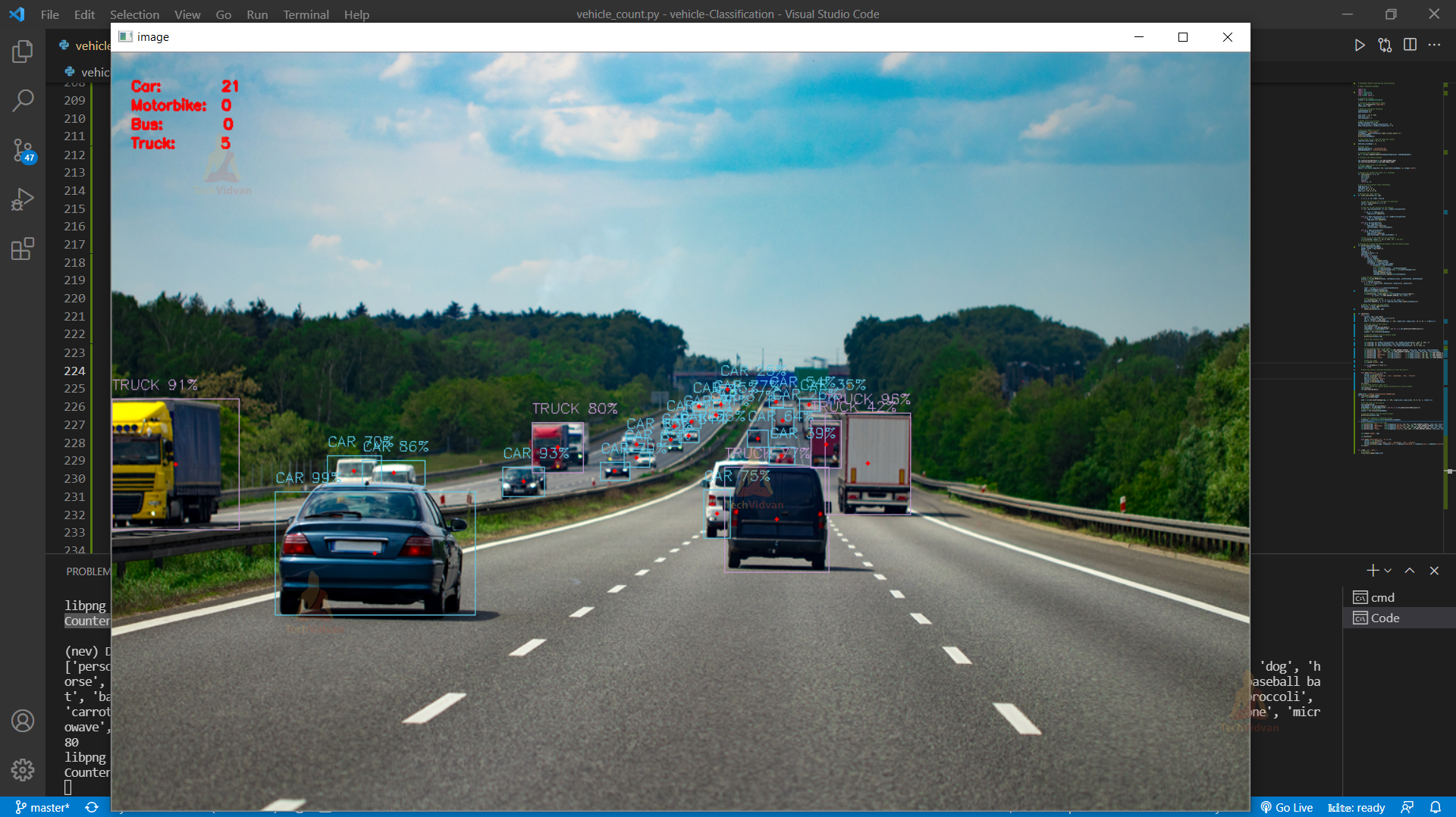
We can see that all the vehicles are successfully detected and have the counting numbers for each detected class.
Summary
In this project, we’ve built an advanced vehicle detection and classification system using OpenCV. We’ve used the YOLOv3 algorithm along with OpenCV to detect and classify objects. And we learned about deep neural networks, file handling systems, and some advanced computer vision techniques.