How to implement the Bootstrapping algorithm in R?

In this article of TechVidvan’s R tutorial series, we will take a look at bootstrapping in statistics. We will learn what bootstrapping is and why we use it in the R programming. Also, we will study how to perform the bootstrap method in R programming.

Bootstrapping is one of the most useful and easy to learn techniques of inferential statistics. So, let’s get cracking!

What is the Bootstrap Method?

Bootstrapping is a technique for inferential statistics. It takes a sample of a single dataset again and again to make many simulated samples. Bootstrapping is useful for calculating statistics like mean, median, standard deviation, confidence intervals, etc. We can summarize the procedure of the bootstrap method as the following:

1. Choose the number of bootstrap samples.

2. Choose the size of each sample.

3. For each sample:

•  If the size of the sample is less than the chosen size, then select a random observation from the dataset and add it to the sample.
• Calculate the given statistic on the sample.

4. Calculate the mean of the calculated sample values.

Methods of Bootstrap

There are two methods of bootstrap:

1. Residual Resampling

In this bootstrap method, we redefine the variables after each resampling. These new residual variables are used to calculate the new dependent variables.

2. Bootstrap Pairs

In this method, pairs of dependent and independent variables are used for sampling. This method can be unstable when working with categorical data but is more robust than residual resampling.

Bootstrapping in R programming

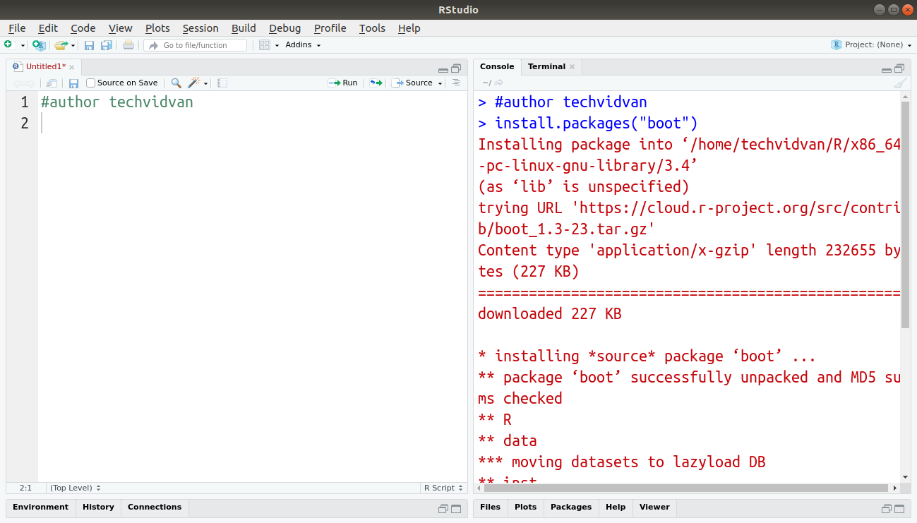
We will use the boot package to use the bootstrap method in R. You can install the package with the following command:

Code:

install.packages("boot")

Output:

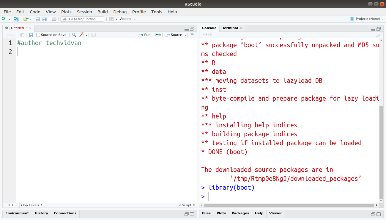
Once installed, you must use the library() function to include the package in your current R session.

Code:

library(boot)

Output:

You can even update the boot package by following the R package tutorial.

Syntax of boot function

The boot package provides us with the boot() function that can perform the bootstrap procedure. The syntax for the boot() function is the following:

boot( data, statistic, R, sim="ordinary", stype=c("i","f","w"), strata=rep(1,n), L=NULL, m=0, weights=NULL, ran.gen=function(d,p)d, mle=NULL, simple=FALSE, ..., parallel=c("no","multicore","snow"),
ncpus=getOption("boot.ncpus",1L), cl=NULL)

Where

1. data can be a vector, matrix or, a data frame.
2. Statistic is the function that is applied to the samples. The arguments given to function depend on the value of the sim argument.
3. R is the number of samples.
4. sim is a character string that indicates the type of simulation required.
5. stype is a character string that shows what the second argument of the statistic represents. Ignored when sim = ”parametric”.
6. strata is an integer vector with the strata for multi-sample problems. Ignored when sim = ”parametric”.
7. L is a vector of influence values. It is only used when sim = “antithetic”.
8. m is the number of predictions for each bootstrap replicate. Only used when sim = “ordinary”.
9. weights is a vector or matrix of importance weights. Only used when sim = “ordinary” or “balanced”.
10. ran.gen is a random number generator function. The first argument to this function is the observed data. It is only used when sim = “parametric”.
11. mle is the second argument passed to the ran.gen function. It is a list of all the objects the ran.gen function will need.
12. simple is a logical value which is TRUE only when sim = “ordinary”, stype = “i”, and, n=0. By default, the boot() function creates an index array for sampling, which is fast but takes memory. When simple = TRUE, the boot() function samples each repetition separately which is slow but uses less memory.
13. ... is for the arguments that have to be passed to the statistic function.
14. parallel is the type of parallel operation to be used (if any).
15. ncups in the number of processes that will run parallelly.
16. cl is an optional parallel or snow cluster for use if parallel = “snow”.

Example of boot function

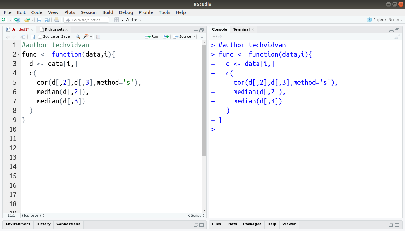
Imagine, we are using the built-in dataset Orange in R. We wish to find the confidence intervals for the median of age, the median of circumference, and spearman’s rank correlation coefficient between these two.

First, we will define a function that calculates the above values from the given dataset.

But before that, you must learn how to write user-defined functions in R.

Code:

func <- function(data,i){
  d <- data[i,]
  c(
    cor(d[,1],d[,2],method=’s’),
    median(d[,1]),
    median(d[,2])
  )
}

Output:

Now, we will use the boot() function to bootstrap the dataset.

Code:

boot1 <- boot(Orange,func,R=1000)
boot1

Output:

The boot() function returns an object of the class “boot”. The original values from the dataset are in the $t₀ element and are the same as the original values in the output. The values calculated in our bootstrap procedure (also called the bootstrap realizations) are in the $t element. The bias values in the output are the difference between the mean of $t (also known as the bootstrap realization of T) and the original values. The std. error in the output is the standard deviation of the bootstrap realizations.

Now, let’s find the confidence intervals or CI for the results. We use the boot.ci() function for this purpose.

Types of Confidence Intervals in Bootstrap

The boot.ci() function of the boot package gives us five types of confidence intervals. These types are:

1. Norm
2. Basic
3. Stud
4. Perc
5. Bca

To understand these types, let us take a look at the following notations first.

Let:

1. The mean of the bootstrap realizations or the bootstrap estimate be t^*.
2. t₀ be a value from the $t₀ that is the original values.
3. The standard error of t* be se*.
4. The bias of the bootstrap estimate be b that is b = t* – t₀.
5. α be a confidence interval, usually α = 0.95.
6. The α-percentile of distribution of $t be θ_α .
7. The 1-α/2-quantile of standard normal distribution be Z_α.

Using the above notations, we can write the various types of CI’s as:

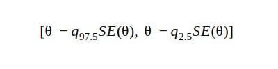
1. Percentile CI

The percentile CI takes the relevant percentile to calculate the confidence intervals.

2. Normal CI

The normal CI is a modification of the Wald CI.

3. Stud CI

In studentized CI, we normalize the distribution of the test statistic, such that it is centered at 0 and has a standard deviation of 1. This corrects for the spread difference and the skew of the original distributin.

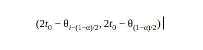
4. Basic CI

The percentile CI gives unreliable results when it comes to weird tail distributions. The basic CI is useful in such cases.

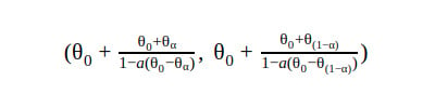
5. Bca CI

BCA stands for bias-corrected, accelerated. The BCA can be unstable when percentiles are outliers and, therefore, extreme in nature.

The following section shows how to calculate each of the CI in R.

The boot.ci() Function

The boot.ci() function is a function provided in the boot package for R. It gives us the bootstrap CI’s for a given boot class object. The object returned by the boot.ci() function is of class "bootci". The function takes a type argument that can be used to mention the type of bootstrap CI required. If the type argument is not used, the function returns all the type of CI’s and gives warnings for whichever it can’t calculate.

Code:

boot.ci(boot1,index=1)

Output:

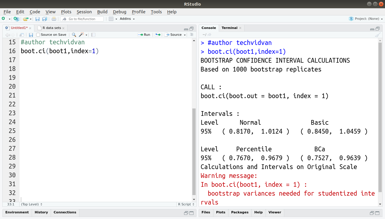
Here, as the function call did not have any type of CI as an argument, the function returned all types of CI.

Summary

Bootstrapping is a statistical technique that is highly useful for inferential statistics. It lets us analyze small samples from a dataset to make predictions about the whole dataset.

In this R tutorial, we learned about the bootstrap method and how to use bootstrapping in R. We learned about the boot packages and its functions. We also learned about the different types of bootstrap CI. Finally, we calculated the confidence intervals for our calculated results.

Any difficulty to implement the Bootstrapping algorithm in R programming?

Ask our TechVidvan experts.

Keep practicing buddy!!