Generalized Linear Models in R – Components, Types and Implementation

Generalized linear models are generalizations of linear models such that the dependent variables are related to the linear model via a link function and the variance of each measurement is a function of its predicted value. In this part of TechVidvan’s R tutorial series, we are going to study what generalized linear models are. We will then take a look at Linear regression, Poisson regression and Logistic regression which are types of GLM in R. Finally, we shall learn how to implement generalized linear models in R.

Generalized Linear Models in R

Generalized linear models are linear models where the response variable is modeled by a linear function of the exploratory variables. GLMs have three components:

• Random component
• Systematic component
• Link function

Let’s see what these components are:

1. Random component

The random component of a GLM is the probability distribution of the response variable.

2. Systematic components

The systematic component includes the exploratory variables that combine to form the linear predictor of the GLM.

3. Link function

The link function includes the link or relation between the random and the systematic components of the GLM. It specifies how the exploratory variables of the linear predictor relate to the values of the response variables.

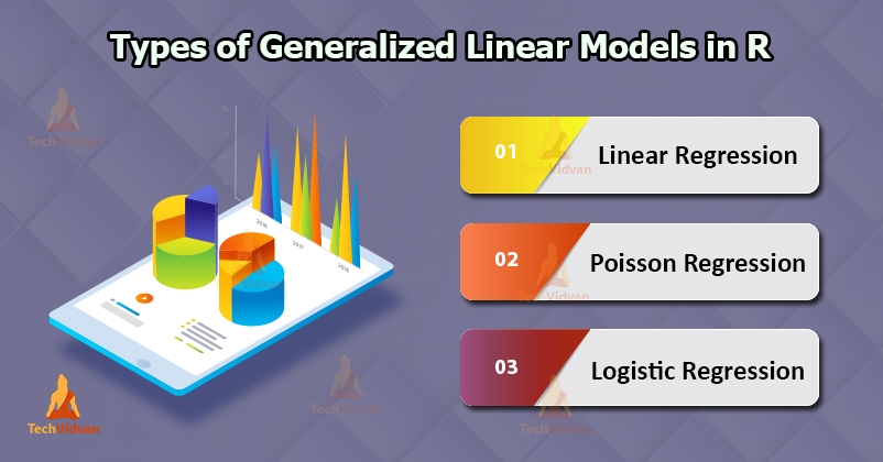
Types of Generalized Linear Models in R

Linear regression, Poisson regression, and Logistic regression are all generalized linear models. Let’s take a look at these on at a time:

1. Linear Regression in R

Linear regression models are used to find a linear relationship between the target continuous variable and one or more predictors. It is used to find the value of the target variable given the values of the exploratory variables.

Linear Regression models can built-in R using the lm() function.

lm(exploratory variable ~ response variable, data)

2. Poisson Regression in R

Poisson models are best suited for discrete non-negative data, unlike linear regression that models continuous data. It allows us to analyze discrete data to isolate exploratory variables that have an effect on a given response variable. We can use the glm() function to build a Poisson model in R by adjusting the family argument to poisson(link = “log”).

glm(exploratory variable ~ response variable, data, family = poisson(link=”log”))

3. Logistic Regression in R

We use Logistic regression to model categorical variables. The outcome of this model is binary in nature. Logistic regression is suitable for situations when the response variable is categorical or logical in nature. We can build a logistic regression model using the glm() function by adjusting the family argument as binomial(link=”logit”).

glm(exploratory variable ~ response variable, data, family = binomial(link=”logit”))

Implementing Generalized Linear Models in R

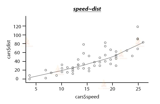
Let us take a look at this with an example. We will be using the car dataset, which is one of the default datasets in R. But, before building the model let us try to understand the data by plotting it.

scatter.smooth(x=cars$speed,y=cars$dist,main="speed~dist")

Output:

To build a linear model, we use the lm() function as follows:

linearMod <- lm(dist~speed, data = cars)
print(linearMod)

Output:

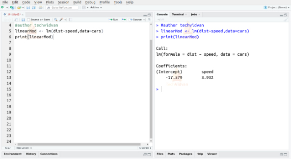
The two coefficients we received, also known as the beta coefficients, give us the formula of the linear equation that defines the relationship between the variables speed and dist.

dist = intercept + beta*speed
D=I+B*S

After building the model, we have to ensure its statistical significance. We do this with the help of the p-value of the model and the individual predictor variables. We can find these p-values by using the summary() function as follows:

summary(linearMod)

Output:

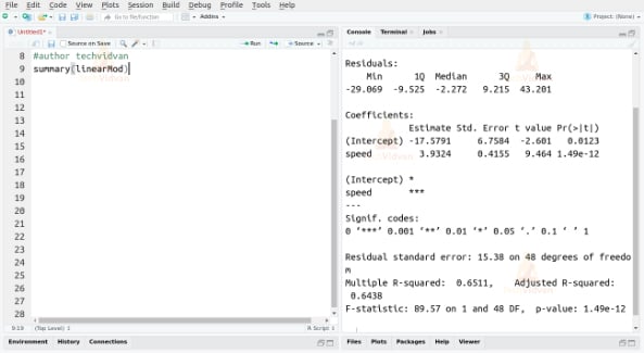
We can consider a linear model to be statistically significant only if both the p-values are less than the pre-determined statistical significance level, which is 0.05 ideally.

Quality of Fit of a GLM in R

There are a few measures that tell how good a fit the GLM is for the given probability distribution. These are:

1. Deviance

Deviance is a measure of the quality or the goodness of the fit of a GLM. A larger value of deviance indicates a bad fit. Deviance measures are usually of two types, Null deviance, and Residual deviance.

The Null deviance shows how well the response variable predicted by a model that includes only the intercept.

The Residual deviance shows the same but when the independent variables are included.

2. Fisher scoring

Fisher scoring uses the Newton-Raphson algorithm to find the best fit for the model. The algorithms first fits the model based on estimate values. It then checks if the model can be improved by using different estimates. This process continues until the algorithm finds that new values will not result in any improvements.

3. Hosmer-Lemeshow test

The Hosmer-Lemeshow test checks the similarities between the model and the observed data. If the difference between the model and the observed data is not significant, we can say that the model has fit well.

4. Akaike Information criterion

The AIC helps in avoiding irrelevant predictors to increase the complexity of the model unnecessarily. Selecting the model with the smallest AIC results in the best fit.

Summary

In this R tutorial of the TechVidvan’s R tutorial series, we learnt about generalized linear models in R or GLM in R. We studied what GLM’s are. We looked at their various types like linear regression, Poisson regression, and logistic regression and also the R functions that are used to build these models. Finally, we saw the implementation of generalized linear models in R with the help of the glm() function.

Do follow us on Facebook to get more articles on latest technologies.