R Random Forest – Ensemble Learning Methods in R

Previously in TechVidvan’s R tutorial series, we learned about decision trees and how to implement them in R. We saw how it is a classification and regression technique and has quite a lot of very important real-life applications.
In this chapter, we are going to learn about the R random forest algorithm and how to implement it.

We will also study ensemble learning methods of machine learning and will then take a look at a few essential machine learning concepts like overfitting, underfitting, bagging, etc.. Finally, we will go through practical implementation of the random forest method in R.

R Random Forest

Random forest is an ensemble learning technique that means that it works by running a collection of learning algorithms to increase the preciseness and accuracy of the results. Random forest works by creating multiple decision trees for a dataset and then aggregating the results. Before we go study random forest in detail, let’s learn about ensemble methods and ensemble theory.

Ensemble Learning Methods

In machine learning, ensemble learning methods are learning algorithms that use multiple learning techniques and algorithms to achieve better results. Ensemble learning methods take more computation than single algorithms. They trade extra computation for improved predictive performance.

Ensemble methods are supervised learning algorithms as they train on data and then make predictions. They tend to be more efficient and accurate when diversity in the component algorithms is more i.e. a collection of random decision trees is better than a collection of entropy-reducing decision trees.

Ensembles are much more flexible in terms of they can represent than singular learning algorithms. This is due to their function being a combination of their component singular algorithms.

Overfitting and Underfitting

A model in machine learning is said to be overfitted when it is overly dependent on data. Such a model corresponds too closely to a particular dataset and therefore will be incorrect when tested on any other data.

Underfitting is the opposite of overfitting. A model is said to be underfitted when it cannot reliably account for the majority of variance in the data. Such a model cannot make reliable predictions about the data it has been trained on.

Overfitting and underfitting are also called overtraining and undertraining.

Bagging

Bagging is an abbreviation for Bootstrapping Aggregating. It is a technique that improves the stability and accuracy of regression and classification algorithms. The biggest advantages and reasons to use bagging are that it reduces variance and helps in avoiding overfitting. Bagging is most commonly used for decision tree algorithms.

Algorithm for R Random Forest Method

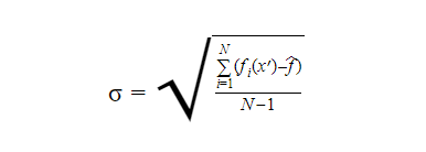
Given a training set X=x1, x2, x3, . . . , xNwith responses Y=y1, y2, y3 . . . , yN. We take random samples from the training set multiple times and fit trees to them. Let f(xi,yi)be the decision tree for the variables xiand yi. Finally, to predict the results for x’ we can average the result of all the trees fi corresponding to x'( in case of continuous ).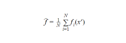In the case of categorical output, the majority output can be chosen. We can calculate an estimation of the uncertainty of the prediction as such:
Generally, the number of trees in a random forest can vary from a few hundred to several thousand depending on the training set. The optimal number of trees can be found by using the cross-validation method.

If one or more features are very strong predictors of the response variable, these features will be in many of the trees which will make these trees correlated. The random forest method employs a technique called feature bagging. This involves selecting a random subset of the features at each candidate split in the learning process. This ensures that the correlation is lower.

Practical Implementation of Random Forest in R

Let us now implement the random forest method in R. We will be using the randomForest and the caTools packages for this. The dataset that we are going to use is a heart disease dataset from the UCI Machine Learning Repository and can be found here.

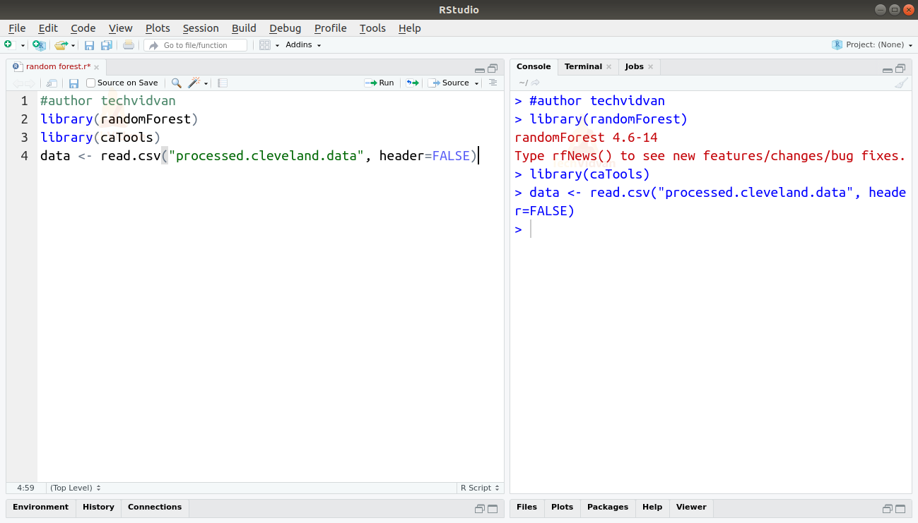
1. Firstly let us begin with loading the packages and the dataset.

library(randomForest)
library(caTools)
data <- read.csv("processed.cleveland.data", header=FALSE)

Output

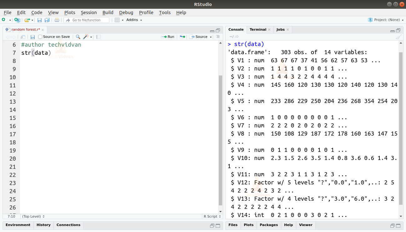
2. Let us now take a look at the data and get familiar with it.

str(data)

Output

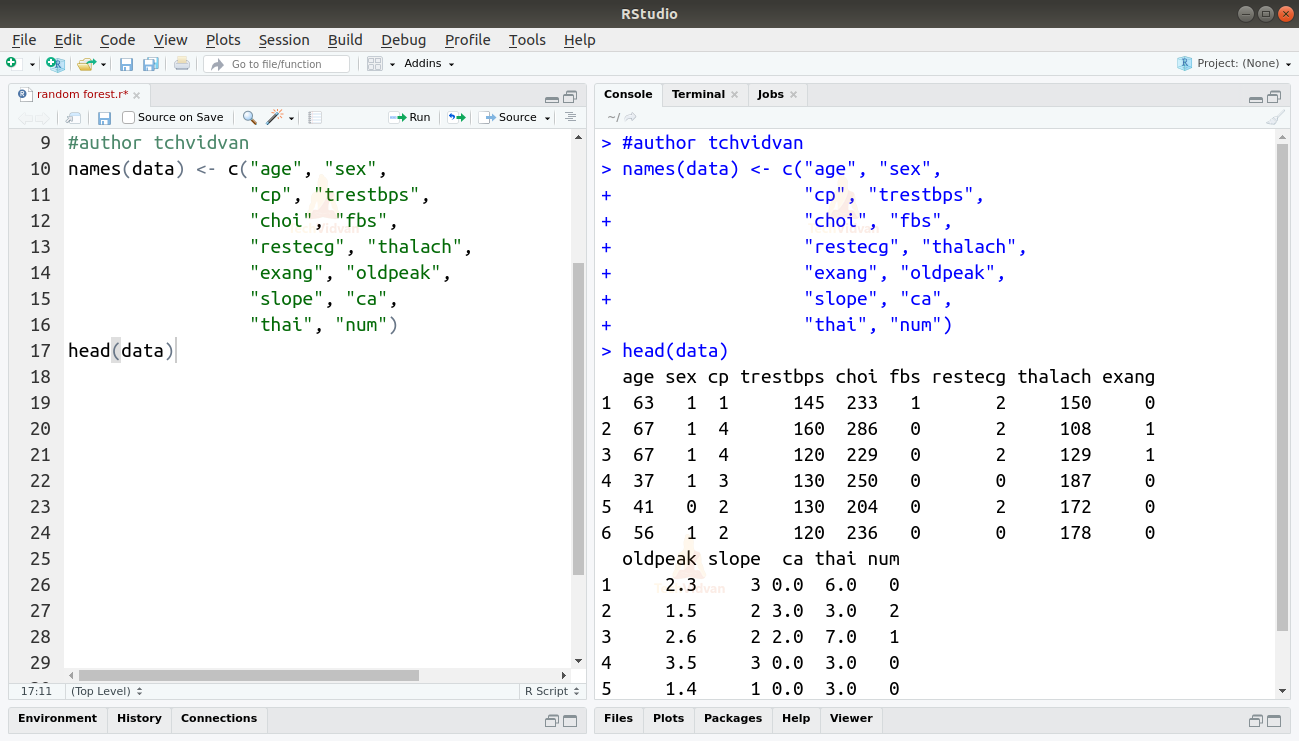
3. As the dataset does not have names to the columns, let’s add some names manually.

names(data) <- c("age", "sex", "cp", "trestbps", "choi", "fbs", "restecg", "thalach", "exang", "oldpeak", "slope", "ca", "thai", "num")
head(data)

Output

4. For simplicity, let’s turn the degree of heart disease into a binary. We will leave the value 0 which indicates an absence of heart disease and replace any value above 1 with 1 which signifies the presence of heart disease. We can also check the class of each column to verify that the categorical variables are stored as such.

data$num[data$num > 1] <- 1
sapply(data,class)

Output

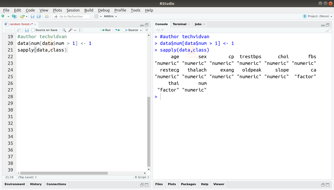
5. As we can see above, the sex variable has a numeric class when it should be a factor. Let us change the class of all the columns to what they should be and also check for missing values. As R expects NA for missing values, it puts a ‘?’ as a placeholder while importing the data. We can use that to find the number of missing values in each column.

data <- transform(data,
                  age=as.integer(age),
                  sex=as.factor(sex),
                  cp=as.factor(cp),
                  trestbps=as.integer(trestbps),
                  choi=as.integer(choi),
                  fbs=as.factor(fbs),
                  restecg=as.factor(restecg),
                  thalach=as.integer(thalach),
                  exang=as.factor(exang),
                  oldpeak=as.numeric(oldpeak),
                  slope=as.factor(slope),
                  ca=as.factor(ca),
                  thai=as.factor(thai),
                  num=as.factor(num)
                )
data[data == "?"] <- NA
colSums(is.na(data))

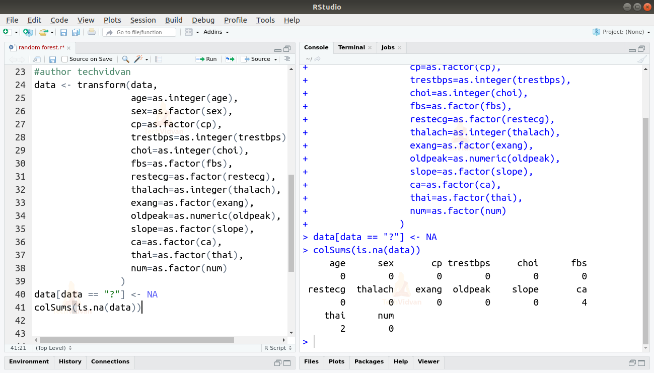
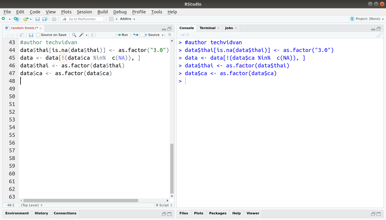
6. Thai has 2 missing values and ca have 4. We know that both thai and ca are factors. For thai, 3 = normal, 6 = fixed defect, and 7 = reversible defect and ca is the number of major vessels (0-3). So let’s replace the NA’s in thai with 3 and we can remove the rows with NA’s in the ca column. We will then cast the columns as factors to remove the “?” as a level from them.

data$thai[is.na(data$thai)] <- as.factor("3.0")
data <- data[!(data$ca %in%  c(NA)), ]
data$thai <- as.factor(data$thai)
data$ca <- as.factor(data$ca)

Output

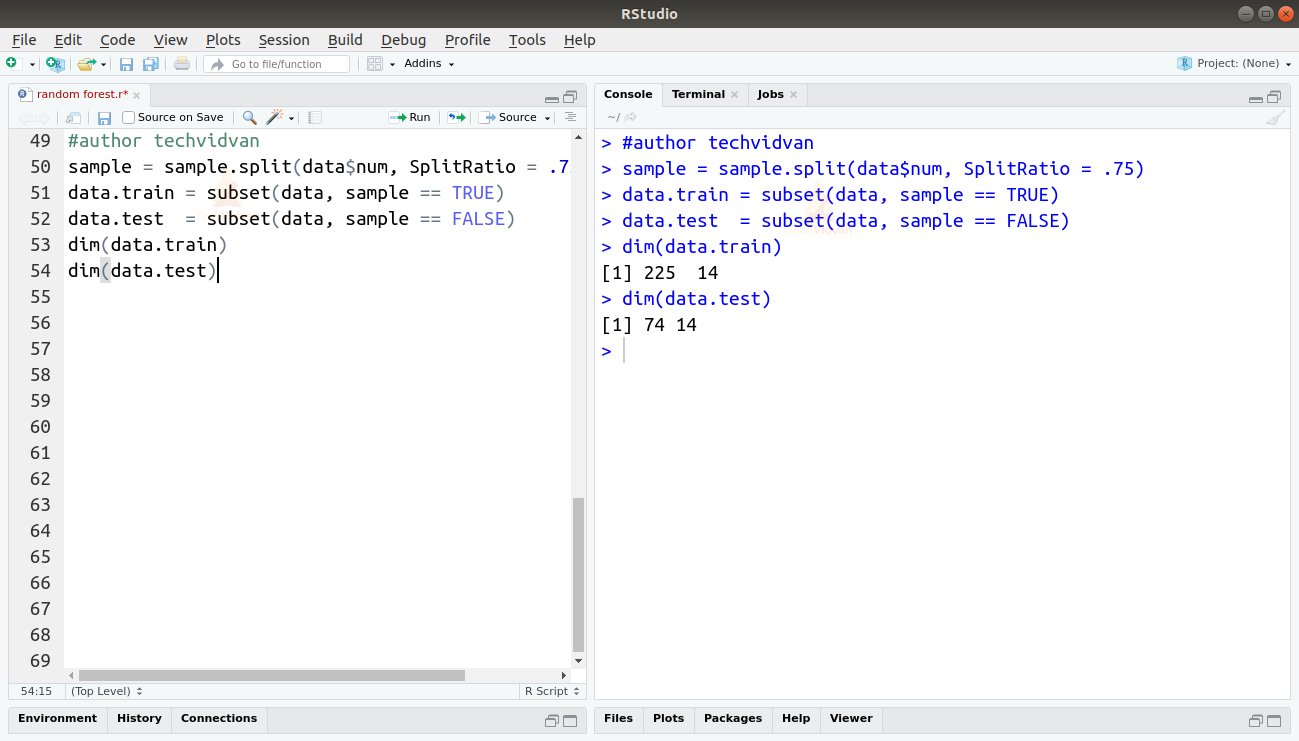
7. Let us now split our data and set some aside for testing.

sample = sample.split(data$num, SplitRatio = .75)
data.train = subset(data, sample == TRUE)
data.test  = subset(data, sample == FALSE)
dim(data.train)
dim(data.test)

Output

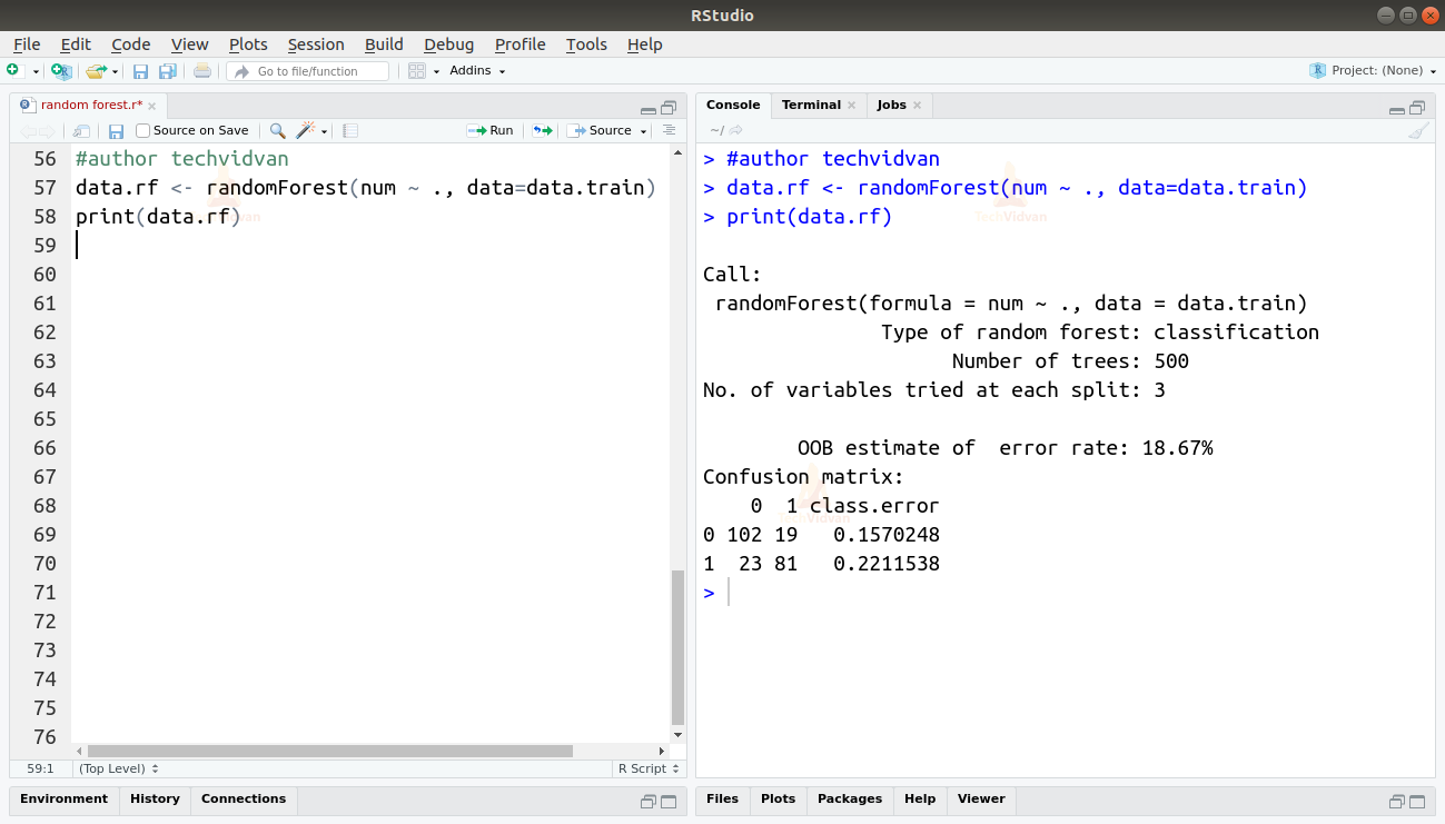
8. Now let’s create our random forest using the randomForest() function.

data.rf <- randomForest(num ~ ., data=data.train)
print(data.rf)

Output

9. Finally let us now predict the test dataset with our model and compare the results.

data.pred <- predict(data.rf, newdata=data.test[-14])
table(data.test[,14],data.pred)

Output

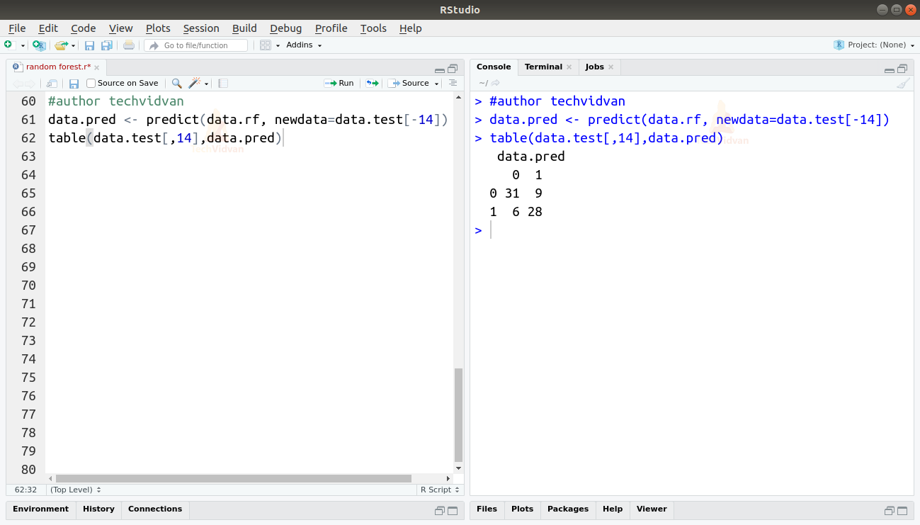
As shown by the table the accuracy of our model is:
                                A=(31+28)/74=0.7980.8

The accuracy is nearly 80%.

Summary

Finally, in this chapter of the TechVidvan’s R tutorial series, we learned about the random forest method. We further studied ensemble methods and then looked at the algorithm of the random forest method. Finally, we saw the practical implementation of the random forest method in R.

Hope the article helped you in learning the concept properly. Do share feedback in the comment section.