AI Search Algorithms Every Data Scientist Must Know

Searching is the fundamental process of each and every AI use case. Within a particular data structure, search algorithms are used for identifying and then extracting relevant information from that data point. One way is by understanding how games work.

Rational agents or Problem-solving agents in AI mostly used these search strategies or algorithms to unravel a specific problem and provide the only result.

In this TechVidvan AI tutorial, we will learn all about AI Search Algorithms.

There are various kinds of games. For example, 3X3 eight-tile, 4X4 fifteen-tile puzzles are the single-operator way of discovering difficulties. As they are comprising a grid of tiles with a clear title.

Therefore, to mastermind the tiles by sliding a tile either vertically or on a level plane into a clear space with the point of achieving some target.

Features of AI Search Algorithms

 

Basic features of a successful search algorithm include:

1. Fulfillment

An inquiry calculation should end on the off chance that it assurances to restore an answer. If, in any event, any arrangement exists for any arbitrary information.

2. Optimality

If an answer saw for a calculation is the best arrangement (most minimal way cost) for an ideal arrangement.

3. Time Complexity

Time multifaceted nature is a proportion of time for a calculation to finish its undertaking.

4. Space Complexity

It is the greatest extra room required anytime during the hunt, as the intricacy of the issue.

Terminologies of AI Search Algorithms

a. Issue Space

Fundamentally, it is the earth where the inquiry happens. (A lot of states and set of administrators to change those states)

b. Issue Instance

It is an aftereffect of Initial state + Goal state.

c. Issue Space Graph

We use it to speak to the issuing state. Additionally, we use hubs to show states and administrators by the edges.

d. The profundity of an issue

We can characterize the length of the shortest possible way.

e. Space Complexity

We can figure it as the most extreme number of hubs put away in memory.

f. Time Complexity

Defined as the most extreme number of hubs that are made.

g. Suitability

We can say it as a property of a calculation to consistently discover an ideal arrangement.

h. Stretching Factor

We can ascertain it as the normal number of youngster hubs in the difficult space diagram.

i. Profundity

Length of the shortest possible way from an underlying state to the objective state.

Types of Search Algorithms in AI

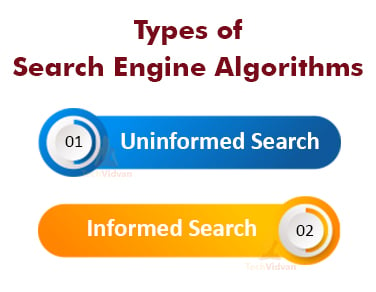
There are two basic types of Search Engine Algorithms namely:

1. Uninformed Search in AI

Uninformed Search Algorithms have no extra data on the objective hub other than the one gave in the difficult definition.

These algorithms don’t have additional information about state or search space aside from the way to traverse the tree, so it’s also called blind search. The designs to arrive at the objective state from the beginning state contrast just by the request and length of activities.

It is more complex to implement than an informed search as there is no utilization of knowledge in uninformed search.

Examples of Uninformed Search are Breadth-First Search, Uniform Cost Search, Depth First Search, Depth Limited Search, Iterative Deepening Depth First Search, Bidirectional Search.

a. Breadth-First Search

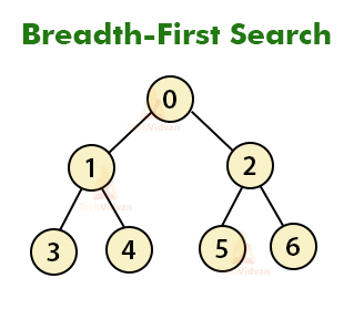
BFS is an algorithm that is utilized to chart information or look through the tree or crossing structures. The calculation productively visits and denotes all the key hubs in a chart in a precise breadthwise design.

BFS may be a traversing algorithm where you ought to start traversing from a specific node. This calculation chooses a solitary hub (starting or source point) in a chart and afterward visits all the hubs neighboring the chosen hub. Keep in mind, BFS gets to these hubs individually.

When the calculation visits and denotes the beginning hub, at that point it moves towards the closest unvisited hubs and examinations them.

Once visited, all hubs are stamped. These emphases proceed until all the hubs of the chart have been effectively visited and checked.

Disadvantages of Breadth-First Search:

• It devours a great deal of memory space. As each degree of hubs is set aside for making the next one.
• Its unpredictability relies upon the number of hubs. It can check copy hubs.

b. Depth First Search

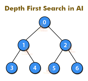
It depends on the idea of LIFO. As it represents Last In First Out. Likewise, actualized in recursion with LIFO stack information structure.

Subsequently, It used to make an indistinguishable arrangement of hubs from the Breadth-First technique, just in the diverse request. As the way is been put away in every emphasis from root to leaf hub.

Consequently, store hubs are direct with space prerequisites. With expanding factor b and profundity as m, the extra room is bm.

Disadvantages of Depth First Search:

• As the calculation may not end and go on limitlessly in one way. Henceforth, an answer to this issue is to pick a cut-off profundity.
• On the off chance that the perfect cut-off is d, and on the off chance that the picked cut-off is lesser than d, at that point this calculation may fall flat.
• If in any case, d is lesser than the fixed cut-off., at that point execution time increments.
• Its multifaceted nature relies upon a number of ways. It can’t check copy hubs.

c. Bidirectional Search

A bidirectional search is a method that as the name suggests, runs two ways. It works with two who look through that run all the while, initial one from source too objective and the other one from objective to source a retrogressive way.

Both searches should compromise the information structure. It relies on a guided chart to locate the most limited way between the source(initial hub) to the objective hub.

The two quests will begin from their individual spots and the calculation stops when the two inquiries meet at a hub. It is a quicker procedure and improves the measure of time required for navigating the diagram.

This methodology is proficient in the situation when the beginning hub and objective hub are one of a kind and characterized. spreading factor is the same for the two.

d. Iterative Deepening Depth First Search

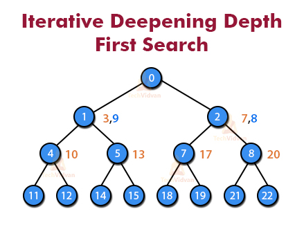
Iterative Deepening Depth First Search (IDDFS) is a search technique wherein iterations of DFS are run continuously with expanding limits until we find the objective.

IDDFS is ideal like BFS, yet utilizes substantially less memory; at every emphasis, it visits the hubs in the inquiry tree in a similar request as profundity first hunt, however, the aggregate request wherein hubs are first visited is adequately expansiveness first.

e. Uniform Cost Search Algorithm in AI

Essentially, it performs arranging in expanding the cost of the way to a hub. Additionally, it consistently grows the least cost hub.

Despite the fact that it is indistinguishable from Breadth-First hunt if each progress has a similar expense. It investigates ways in the expanding request of cost.

Disadvantages of Uniform Cost Search Algorithm:

• There can be numerous long ways with the expense ≤ C*.
• Uniform Cost search must investigate them all.

2. Informed Search in AI

Informed Search Algorithms have data on the objective state which helps in progressively proficient looking. This data collected as a capacity that gauges how close a state is to the objective state.

Its major advantage is that it is efficiency is high and is capable of finding solutions in a shorter duration than uninformed Search.

It is also comparatively less expensive than an informed search.

Types of AI Informed Search Algorithms

Informed search in AI is of multiple types as below:

a. Greedy Best First Search

This type of search consistently chooses the way which shows up best at that point. It is the mix of profundity first inquiry and expansiveness first hunt calculations. It utilizes heuristic capacity and searches. The BFS permits us to take the benefits of the two calculations.

With the assistance of the best-first hunt, at each progression, we can pick the most encouraging hub. In the BFS calculation, we grow the hub which is nearest to the objective hub and the nearest cost by the heuristic search.

The major benefit of this is that it combines the advantages of both BFS and DFS.

b. A*Search

A* search is the most regularly known type of best-first pursuit. It utilizes heuristic capacity h(n), and cost to arrive at the hub n from the beginning state g(n). It has consolidated highlights of UCS and avaricious best-first inquiry, by which it take care of the issue proficiently.

A* search calculation finds the briefest way through the hunt space utilizing the heuristic capacity.

This hunt calculation extends fewer pursuit trees and gives an ideal outcome quicker. A* calculation is like UCS aside from that it utilizes g(n)+h(n) rather than g(n).

Heuristic Evaluation Functions

They find the resources spent in the shortest possible way between two states.

A heuristic search for sliding-tiles games is registered by checking a number of moves that each tile makes from its objective state and including these number of moves for all tiles.

Pure Heuristic Search: Pure Heuristic Search is the easiest of heuristic search methods. It grows by hubs arranged by their heuristic qualities h(n).

It keeps up a shut rundown of those hubs that have just extended, and an open rundown of those hubs that have produced however not yet extended.

The calculation starts with simply the underlying state on the open rundown. At each cycle, a hub on the open rundown with the base h(n) esteem extended, producing the entirety of its subsets and is set on the shut rundown.

The heuristic search on the subsets is put up on the open rundown by their heuristic qualities. The calculation proceeds until we reach an objective state is for an extension.

Brute Force Strategies

This procedure doesn’t require any area explicit information. Along these lines, it’s so straightforward system. Thus, it works easily and fine with few potential states.

Necessities for Brute Force Algorithms are:

• State portrayal
• A lot of legitimate administrators
• Beginning state
• Objective state portrayal

Local Search Algorithms in AI

1. Hill Climbing in AI

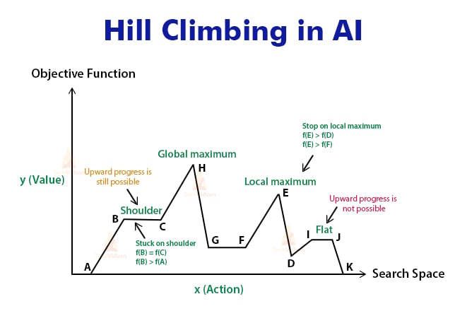
Hill Climbing is a heuristic quest for scientific advancement issues in the field of Artificial Intelligence.

Given an enormous arrangement of information sources and a decent heuristic capacity, it attempts to discover an adequately decent answer for the issue. This arrangement may not be the worldwide ideal greatest.

‘Heuristic search’ implies that this pursuit calculation may not locate the ideal answer for the issue. Nonetheless, it will give a decent arrangement in a sensible time.

A heuristic capacity is a capacity that will rank all the potential choices at any expanding step in search calculation dependent on the accessible data. It causes the calculation to choose the most ideal course out of courses.

Hill Climbing is further classified as:

• Simple Hill Climbing
• Steepest Ascent Hill Climbing
• Stochastic Hill Climbing

2. Local Beam Search Algorithm in AI

In this calculation, we need to hold k number of states at some random time. Toward the start, we need to created states arbitrarily.

In addition, with the goal work, we need to process replacements of these k states. Additionally, this stop, if any of these replacements is the greatest estimation of the goal work.

Else, we need to put the (underlying k states and k number of replacements of the states = 2k) states in a pool. Additionally, a pool is arranged numerically.

Further, we need to choose the most noteworthy k states as new introductory states. This procedure proceeds until we reach the most extreme end.

Work Beam Search( issue, k), restores an answer state.

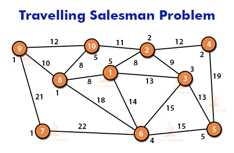
Travelling Salesman Problem in AI:

The traveling salesman problem poses the underlying question that: “When cities with the distance between each pair of them provided, the main objective is to find out the shortest route from City A to B.” Look at the figure for reference.

Start
Discover all (n – 1)! Potential arrangements, where n is the all outnumber of urban communities. Further, decide the base expense by discovering the expense of each of these (n – 1)! arrangements. At long last, keep the one with the lowest amount of money spent.
End

Simulated Annealing

A technique that involves warming and cooling metal to change its inner structure for altering its physical properties is known as annealing.

At the point when the metal cools, its new structure is seized, and the metal holds its recently gotten properties. In the Simulated Annealing Process, the temperature is not fixed.

We at first set the temperature high and afterward permit it to ‘cool’ gradually as the calculation continues. At this point when the temperature is high, the calculation permits optimally lesser solutions.

Summary

Basically, we have contemplated Popular Search Algorithms in AI. The ones susceptible to be touched by the transformation are the repetitive, manual tasks that do not require great capacity but that can be moderately simple optimized.

We hope this article covers most of if not all the popular search algorithms in AI.