Clustering in Machine Learning

In this article, we will study about an unsupervised learning-based technique known as clustering in machine learning.Here, we will discuss what clustering really is, What are its types? And we will look at the algorithms involved in the clustering technique.

Clustering in Machine Learning

Let’s try to understand what clustering exactly is. Examples make the job a lot more easier.

So, as we know, there are two types of learning: active and passive.

Passive means that the model follows a certain pre-written path and is also done under supervision. This doesn’t mean something like we will take unsupervised learning on the active side. It is just that the human intervention in unsupervised learning is quite minimal as compared to supervised learning.

Also, we have unlabeled data in unsupervised learning. So, here, the algorithm has to completely analyze the data, find patterns, and cluster the data depicting similar features.

For example, if we provide a dataset consisting of images of two different objects. The model will scan the images for certain features. If some images have matching features, it will form a cluster.

Note:-Active learning is a different concept. It’s applicable for semi-supervised and reinforcement learning techniques.

Examples of Clustering in Machine Learning

A real-life example would be: -Trying to solve a hard problem in chess. The possibilities to checkmate the king are endless. There is no predefined or pre-set solution in chess. You have to analyze the positions, your pieces, the opponent’s pieces and find a solution.

These traits to find the solution are the dataset, you are the model that has to analyze and find the answer. This is what unsupervised learning is.

Now let’s understand clustering. In clustering, we classify data points into clusters based on similar features rather than labels. The labelling part in clustering comes at the end when clustering is over.

Also, we should add a lot of data to the dataset, to increase the accuracy of the results. The algorithm will learn various patterns in the dataset.

Like, it will look for certain traits and features and compare the similarities between the data.

There is a difference here between classification and clustering. The labeling part involves a lot of human intervention that proves both costly and time-consuming. Although labelling gets fairly simple in unsupervised learning, the model would have to process more due to more analysis.

Let’s take an example. If we have a dataset consisting of images of tigers, zebras, leopards, cheetahs.

The clustering algorithm would analyze this dataset and then divide the data based on some specific characteristics. The characteristics would include fur color, patterns (spots, stripes), face shape, etc.

The model would remember the pattern in which it classified the data. This knowledge will come in handy for future unknown data.

We also have other applications of clustering like fake-news detection, fraud detection, spam mail segregation, etc. Now, let’s dive a bit deeper into clustering now that we have seen and understood it.

There are various types of clustering that we should know about. These will help us to further classify and understand the various algorithms that unsupervised learning has.

These include:

• Centroid-based clustering
• Density-based clustering
• Distribution-based clustering
• Hierarchical clustering
• Grid clustering

Now let’s understand these one-by-one.

Types of Clustering in Machine Learning

1. Centroid-Based Clustering in Machine Learning

In centroid-based clustering, we form clusters around several points that act as the centroids. The k-means clustering algorithm is the perfect example of the Centroid-based clustering method. Here, we form k number of clusters that have k number of centroids.

The algorithm assigns the datapoints to certain cluster centres (centroids) based on their proximity to certain centroids.

The algorithm measures the Euclidean distances between the datapoints and all k centroids. The one that is the nearest will get clustered with that particular centroid.

Also, k-means is the most widely used centroid-based clustering algorithm. The primary aim of the algorithm is to simplify an N-dimensional dataset into smaller K clusters.

K-means Clustering in Machine Learning

Let’s try to understand more about k-means clustering. It is an iterative clustering type of algorithm. This means that it compares each datapoint’s proximity with the centroids one-by-one in an iterative fashion. The premise of this algorithm is that it has to find the maximum (local maxima) or the best possible value for each iteration.

Let’s understand the working of the algorithm with the help of some images:

Let’s say we have two different types of datapoints. Red colour and blue colour.

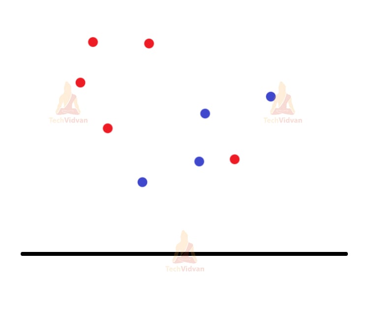
Now, for the next step, let’s assign the value of k. Let’s say k=2 as we have two types of data. K=2 means we will have two centroids far from each other

Note:- The centroids should always remain distant from each other to avoid any confusion and error.

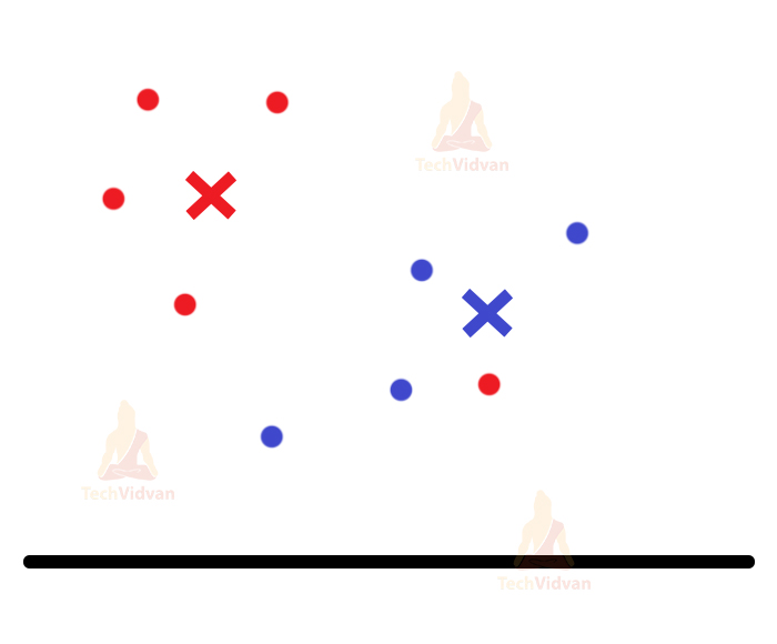
The two-colored crosses are the centroids.

Now the algorithm will compare the distance of each point with the centroids. The points will join the cluster whose centroid is nearer to them. This algorithm makes nice use of the distance metrics for this purpose. The points are now assigned to their respective clusters.

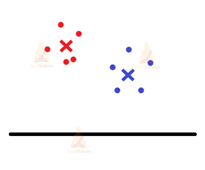
After this, again centroids are assigned for the clusters and again they re-adjust themselves.

The last two steps will keep on continuing until the algorithm achieves maximum accuracy (maxima) or you can say, until the clusters stop moving and everything becomes stable.

So, let’s see the coding part of it:

Step 1: First, we will import all the necessary libraries. We have the basic import libraries:

from sklearn.datasets import make_classification
from sklearn.cluster import KMeans
from matplotlib import pyplot
from numpy import unique
from numpy import where

Here, make_classification is for the dataset. KMeans is to import the model for the KMeans algorithm.

If there are any special or unique elements in the NumPy array, we can extract them with the help of the unique function provided by the unique library. Also, in the case of the where function, you can relate it with the conditional operator in mathematics.

You have to give a condition to the where function in order to get the output according to it. Remember that these two functions belong to the Numpy group.

Here, we have used sklearn.datasets in order to include more parameters related to the datasets.

Step-2: Let’s try to define the dataset. We will use the make_classification function to define our dataset and to include certain parameters with it.

A, _ = make_classification(n_samples=1000, n_features=4, n_informative=2, n_redundant=0,  n_repeated=0, n_clusters_per_class=1, random_state=4)

Remember that, whatever parameter you choose to have, the output would look different for each case.

Also, these parameters have specific meanings.

n_samples is the number of samples.

n_features is the number of features that you would want to have in the dataset.

Now, these next three are a bit important to know. As they are responsible for how your data would look.

n_informative tells the number of important and informative features of your data.

n_redundant gives you random combinations of informative features.

n_repeated helps to draw out the duplicate features from the above two features.

The Numpy array stores the features in the same order as mentioned and Random_state helps in giving random numbers in the same order.

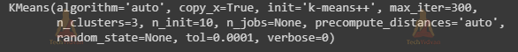
Step-3: Now, we will bring in our model. In the parameter of our model or the function name (KMeans), we will give the number of clusters we need:

model = KMeans(n_clusters=3)

Step-4: Now, here we run the model. We try to fit in the data that we have defined above.

model.fit(A)

After execution, it will also show a certain output message (depends on the framework that you use)

Step-5: The function predict() will help to analyze and predict the dataset to make clusters.

B = model.predict(A)

Step-6: Here the unique function comes into play. This will help to segregate certain features for the cluster in a NumPy array.

clust = unique(B)

Step-7: Now, we will run the entire system in a loop so as to keep taking the next set of data for creating the clusters. Here, the clust variable already has the segregated data for the cluster.

We will use it in the where function and create a condition.

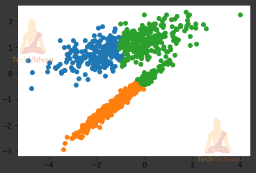
In the end, we will see a graph plotted as a result (because pyplot and matplotlib come into play here).

for cluster in clust:
    C = where(B == cluster)
    pyplot.scatter(A[C, 0], A[C, 1])
pyplot.show()

2. Density-Based Clustering in Machine Learning

In this type of clustering, the clustering doesn’t happen around centroid or central points, but the cluster forms where the density looks higher. Also, the advantage is that unlike centroid-based clustering it doesn’t include all the points.

Including all the points can create unnecessary noise in the data and that is where density-based clustering has an edge over centroid-based clustering.

The sparse/noise datapoints are included in order to define the border between clusters. These points are always outside the main cluster.

Also, one negative thing is that in density-based clustering, the cluster borders are defined by decreasing density. So, the borders might be of varied shapes that make it difficult to draw a perfect border for clusters. However, there are many methods out there to improve these kinds of problems, but we look at them some other time.

We have three main algorithms in Density-based clustering – DBSCAN, HDBSCAN, and OPTICS.

DBSCAN uses a fixed distance for separating the dense clusters from the noise datapoints. It is the fastest among clustering algorithms.

HDBSCAN uses a range of distances to separate itself from the noise. It requires the least amount of user-input.

OPTICS measures the distance between neighboring features and it draws a reachability plot to separate itself from the noise datapoints.

Now, we will use the same code but some different functions to understand density-based clustering. So, we will only mention the different functions here as the rest is the same.

So, let’s have a look at DBSCAN: We just need to import DBSCAN:

from sklearn.cluster import DBSCAN

This will import the DBSCAN model into your program. Now to define your model and to provide it with the arguments:

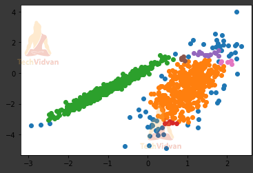
model = DBSCAN(eps=0.20, min_samples=5)

Here, eps is the max. distance between two data points. This is the prime parameter for the DBSCAN as the values we enter in eps would change the plot every time.

The reason is that cluster density would look different for different values.

Also, min_samples helps to set the minimum number of samples we want within a neighborhood collection of features. So, the output for the given value set would be:

3. Distribution-Based Clustering in Machine Learning

In distribution-based clustering, if the distance between the point and the central distribution of points increases, then the probability of the point being included in the distribution decreases.

For problems like these, we use the Gaussian distribution model. The model works like, there will be a fixed number of distributors for the Gaussian model. These distributors are concentric figures with decreasing color intensity from inside to the outside.

The central part tends to be denser and it tends to decrease as we go outside as we have bigger distributors now. So, even though distributors might contain the same number of points, their densities may still differ due to the size of distributors. Overfitting can be a bit of a problem for this type of clustering.

As long as we don’t set any strong criteria for points, we can avoid overfitting.

The Gaussian mixture model is generally used with the expectation-maximization model. An important point to remember that we cannot use this technique for density-based clustering as it would not properly fit among the distributions.

Only expectation-maximization algorithms can work well with Gaussian mixture models.

So let’s see how the Gaussian distribution looks in general:

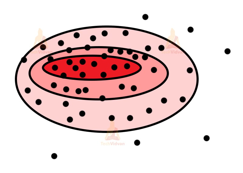
The concentric figures may not be this perfect, but it’s a similar depiction of what the real thing looks like.

Now, let’s understand the code involved in this:

The code has numerous similarities just like the previous case. So, we will only mention the main components involved as the rest gets pretty much the same. These are all easier examples, just to understand how the clustering works.

The coding has an enormous depth with numerous parameters for the functions that we use. But, here we restrict to very few functions to make the explanation simpler.

From sklearn.cluster import GaussianMixture

Firstly, we will import the model.

Note: All the models and algorithms that are a part of sklearn, we can import them directly from sklearn and just use their function to define the models.

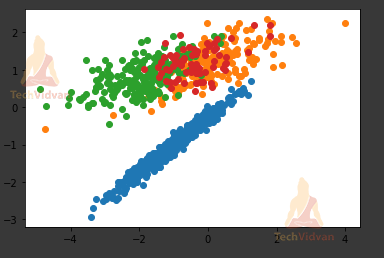
model = GaussianMixture(n_components=4)

Here, n_components is the number of mixture components ( the number of different colored components that we will use in the plot).

So, the result would look like:

4. Hierarchical Clustering in Machine Learning

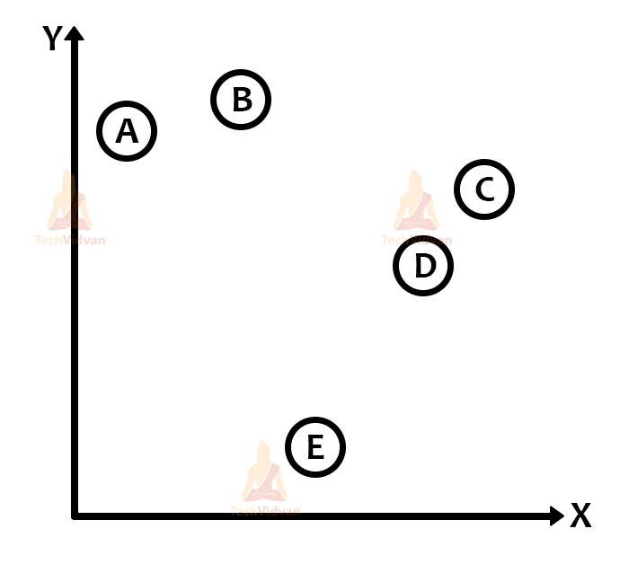
Well, in hierarchical clustering we deal with either merging of clusters or division of a big cluster.

So, we should know that hierarchical clustering has two types: Agglomerative hierarchical clustering and divisive hierarchical clustering.

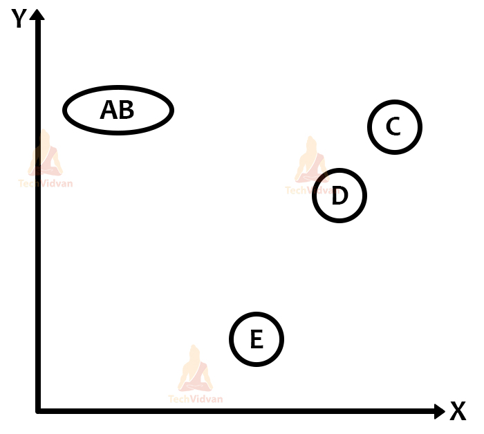
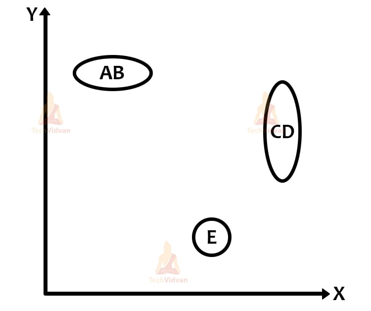
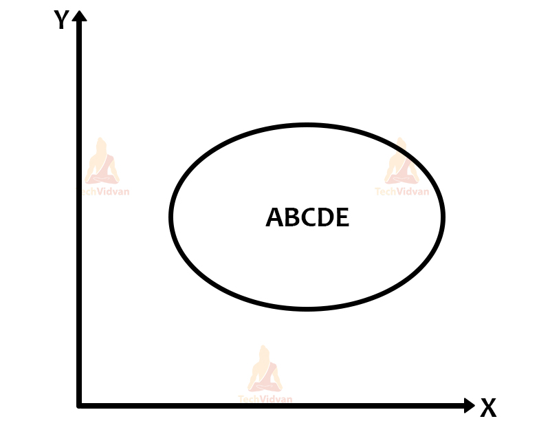
In agglomerative clustering, we tend to merge smaller clusters into bigger clusters. But this also has some process. If the two clusters that we compare have similarities between them and if they are near to each other, then we merge them.

In the case of divisive hierarchical clustering, we divide one big cluster into n-smaller clusters. The clusters here are divided if some datapoints are not similar to the larger cluster; we separate them and make an individual cluster for them.

For solving the hierarchical clustering problem, we use the proximity (distance) matrix in which we store the distances of each individual cluster among each other.

For every merge or divide, the matrix would change because at every next step we get a new cluster.

Like, if we have 5 clusters, we merge two of them, then the matrix will then have 4 clusters and the distances stored in the matrix will eventually change (Same case for divisive hierarchical clustering as well).

Also, for visualizing hierarchical clustering, we use a dendrogram, which is a type of graph. In hierarchical clustering, the most important job is to calculate the similarity between clusters.

It’s the most important part as it helps us to understand whether to merge or divide the cluster. We have several methods like:

Single Linkage Algorithm (MIN)

• In this, we take two points from two individual clusters and these points have to be the closest to each.
• We then calculate the distance and similarity between them.
• It works well for separating non-elliptical clusters.
• Noise in the data can create problems.

Complete Linkage Algorithm (MAX)

• This is the exact opposite of the MIN algorithm.
• We take the distance between the two farthest points in two clusters and measure the distance and similarities.
• It works well even in the presence of noise.
• However, it can accidentally break bigger clusters as well.

Group Average

• Here, we take all the points and then measure them.
• It can accurately separate clusters even if there remains noise in between clusters.

Distance Between the Centroids

• We can measure the distance between the centroids of both the clusters.
• Although it’s not used that much as you have to find the centroid after every merge or divide.

Ward’s Method

• This one is the last method to calculate the similarity.
• Here, instead of taking the average, we take the sum of squares of distances.

Note:- The complexity of space in hierarchical clustering is O(n2). We require lots and lots of space to hold the matrix. For time complexity it is O(n3). The iterations we perform can get complex if there is a large dataset.

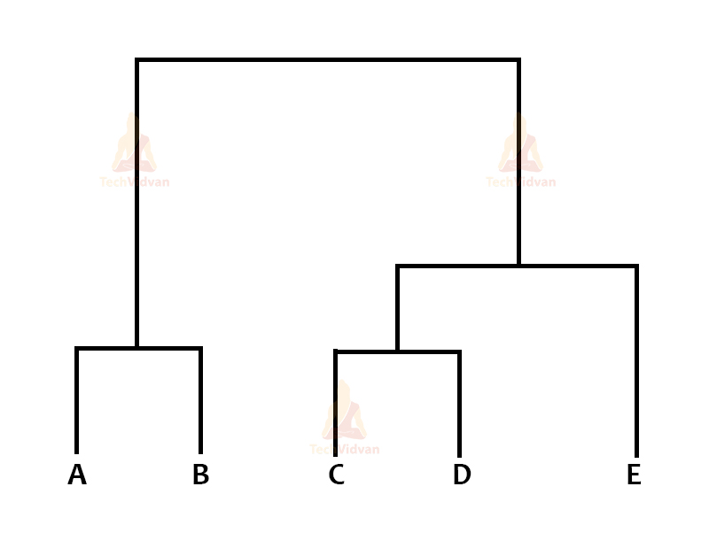
We have some visual representations of how the clustering happens in hierarchical clustering:

There is also the proximity matrix and the dendrogram:

This is the proximity matrix. Now the dendrogram:

5. Grid Clustering in Machine Learning

This technique is very useful for multidimensional spaces. Here, we can divide the entire data space into a finite number of small cells. This helps a lot in reducing the complexity of the problem and this is what separates grid clustering from all conventional clustering.

We can recognize denser areas as the places that have clusters. When we divide the plane into cells, we can then calculate the density of each cell and then sort them.

At first, we will select one cell and calculate its density. If it is more than the normal density it will become a cluster. We will apply the same process for the cell’s neighbors until there are no neighbors left. All the neighboring cells would have grouped into a cluster. The process will continue until all the cells are traversed.

Here, we focus on the cells rather than the data. This helps in reducing complexity. The algorithms that fall under the grid-based clustering are the STING and CLIQUE algorithms.

Applications of Clustering in Machine Learning

So, finally, let’s have a look at the specific areas where this concept is applied. Here are the top applications of the clustering concept:

• It’s useful in various image recognition platforms and also various image segregation tasks. One such example is the biological field.
• Here, this can help the researchers to categorize and classify certain unknown species.
• Clustering can come in handy for the city’s crime branch for classifying different parts of a city based on the crime-rate.
• The algorithm can classify and tell based on the frequency and number of cases that, which part has more criminal activities.
• It’s quite useful in data-mining as well because clustering can help in understanding the data.
• It can be useful for banks as a fraud detection algorithm. The bank sector faces a problem of credit card scams and frauds.
• Using clustering we can uncover several hidden patterns that may tell us which scheme is a fraudulent scheme.
• We can understand various seismic zones based on the data and the clustering algorithm can create clusters of various seismic activities and active regions.
• In the health industry as well, we can use this algorithm to detect various ailments, especially tumors and cancers.
• The search engine is a prime example of the clustering technique.
• It categorizes search results on the basis of billions of searches and has the results ready at the go every time for every search.
• It can be of great use in analyzing data of soil for agriculture.
• With the data of the soil it can classify whether the soil has the necessary nutrient content for growing crops.
• It is also useful in the case of advertising the product based on customer interest and feedback.

Conclusion

So, for this article, we have studied all the necessary aspects of clustering in machine learning that especially a student or someone who wants to pursue ML should know about.

We covered everything from what clustering is to what are its types. We even have a few coding examples, more importantly, what function and library we should use in ML is more important than to understand the whole code. You can understand the whole code if you know python language.

We even saw the algorithms that fall under various categories. Also, several diagrams have been used for better understanding.