Top 10 Data Science Algorithms You Must Know About

The implementation of Data Science to any problem requires a set of skills. Machine Learning is an integral part of this skill set.

For doing Data Science, you must know the various Machine Learning algorithms used for solving different types of problems, as a single algorithm cannot be the best for all types of use cases. These algorithms find an application in various tasks like prediction, classification, clustering, etc. from the dataset under consideration.

In this article, we will see a brief introduction to the top Data Science algorithms.

Top Data Science Algorithms

The most popular Machine Learning algorithms used by the Data Scientists are:

1. Linear Regression

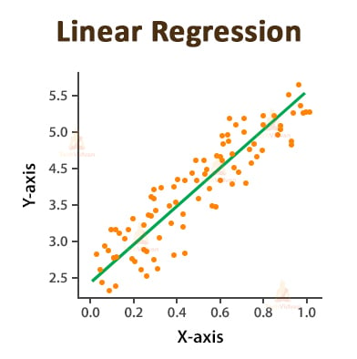
Linear regression method is used for predicting the value of the dependent variable by using the values of the independent variable.

The linear regression model is suitable for predicting the value of a continuous quantity.

OR

The linear regression model represents the relationship between the input variables (x) and the output variable (y) of a dataset in terms of a line given by the equation,

y = b0 + b1x

Where,

• y is the dependent variable whose value we want to predict.
• x is the independent variable whose values are used for predicting the dependent variable.
• b0 and b1 are constants in which b0 is the Y-intercept and b1 is the slope.

The main aim of this method is to find the value of b0 and b1 to find the best fit line that will be covering or will be nearest to most of the data points.

2. Logistic Regression

Linear Regression is always used for representing the relationship between some continuous values. However, contrary to this Logistic Regression works on discrete values.

Logistic regression finds the most common application in solving binary classification problems, that is, when there are only two possibilities of an event, either the event will occur or it will not occur (0 or 1).

Thus, in Logistic Regression, we convert the predicted values into such values that lie in the range of 0 to 1 by using a non-linear transform function which is called a logistic function.

The logistic function results in an S-shaped curve and is therefore also called a Sigmoid function given by the equation,

?(x) = 1/1+e^-x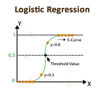

The equation of Logistic Regression is,

P(x) = e^(b0+b1x)/1 + e^(b0+b1x)

Where b0 and b1 are coefficients and the goal of Logistic Regression is to find the value of these coefficients.

3. Decision Trees

Decision trees help in solving both classification and prediction problems. It makes it easy to understand the data for better accuracy of the predictions. Each node of the Decision tree represents a feature or an attribute, each link represents a decision and each leaf node holds a class label, that is, the outcome.

The drawback of decision trees is that it suffers from the problem of overfitting.

Basically, these two Data Science algorithms are most commonly used for implementing the Decision trees.

• ID3 ( Iterative Dichotomiser 3) Algorithm

This algorithm uses entropy and information gain as the decision metric.

• Cart ( Classification and Regression Tree) Algorithm

This algorithm uses the Gini index as the decision metric. The below image will help you to understand things better.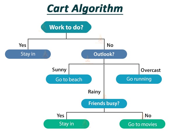

4. Naive Bayes

The Naive Bayes algorithm helps in building predictive models. We use this Data Science algorithm when we want to calculate the probability of the occurrence of an event in the future.

Here, we have prior knowledge that another event has already occurred.

The Naive Bayes algorithm works on the assumption that each feature is independent and has an individual contribution to the final prediction.

The Naive Bayes theorem is represented by:

P(A|B) = P(B|A) P(A) / P(B)

Where A and B are two events.

• P(A|B) is the posterior probability i.e. the probability of A given that B has already occurred.
• P(B|A) is the likelihood i.e. the probability of B given that A has already occurred.
• P(A) is the class prior to probability.
• P(B) is the predictor prior probability.

5. KNN

KNN stands for K-Nearest Neighbors. This Data Science algorithm employs both classification and regression problems.

The KNN algorithm considers the complete dataset as the training dataset. After training the model using the KNN algorithm, we try to predict the outcome of a new data point.

Here, the KNN algorithm searches the entire data set for identifying the k most similar or nearest neighbors of that data point. It then predicts the outcome based on these k instances.

For finding the nearest neighbors of a data instance, we can use various distance measures like Euclidean distance, Hamming distance, etc.

To better understand, let us consider the following example.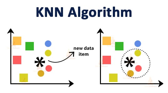

Here we have represented the two classes A and B by the circle and the square respectively.

Let us assume the value of k is 3.

Now we will first find three data points that are closest to the new data item and enclose them in a dotted circle. Here the three closest points of the new data item belong to class A. Thus, we can say that the new data point will also belong to class A.

Now you all might be thinking that how we assumed k=3?

The selection of the value of k is a very critical task. You should take such a value of k that it is neither too small nor too large. Another simpler approach is to take k = √n where n is the number of data points.

6. Support Vector Machine (SVM)

Support Vector Machine or SVM comes under the category of supervised Machine Learning algorithms and finds an application in both classification and regression problems. It is most commonly used for classification of problems and classifies the data points by using a hyperplane.

The first step of this Data Science algorithm involves plotting all the data items as individual points in an n-dimensional graph.

Here, n is the number of features and the value of each individual feature is the value of a specific coordinate. Then we find the hyperplane that best separates the two classes for classifying them.

Finding the correct hyperplane plays the most important role in classification. The data points which are closest to the separating hyperplane are the support vectors.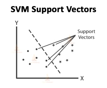

Let us consider the following example to understand how you can identify the right hyperplane.

The basic principle for selecting the best hyperplane is that you have to choose the hyperplane that separates the two classes very well.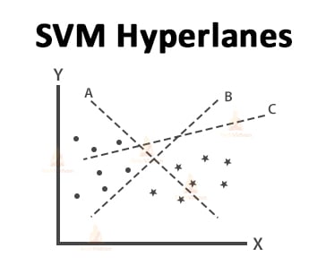

In this case, the hyperplane B is classifying the data points very well. Thus, B will be the right hyperplane.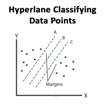

All three hyperplanes are separating the two classes properly. In such cases, we have to select the hyperplane with the maximum margin.

As we can see in the above image, hyperplane B has the maximum margin therefore it will be the right hyperplane.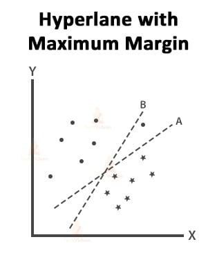

In this case, the hyperplane B has the maximum margin but it is not classifying the two classes accurately. Thus, A will be the right hyperplane.

7. K-Means Clustering

K-means clustering is a type of unsupervised Machine Learning algorithm.

Clustering basically means dividing the data set into groups of similar data items called clusters. K means clustering categorizes the data items into k groups with similar data items.

For measuring this similarity, we use Euclidean distance which is given by,

D = √(x1-x2)^2 + (y1-y2)^2

K means clustering is iterative in nature.

The basic steps followed by the algorithm are as follows:

• First, we select the value of k which is equal to the number of clusters into which we want to categorize our data.
• Then we assign the random center values to each of these k clusters.
• Now we start searching for the nearest data points to the cluster centers by using the Euclidean distance formula.
• In the next step, we calculate the mean of the data points assigned to each cluster.
• Again we search for the nearest data points to the newly created centers and assign them to their closest clusters.
• We should keep repeating the above steps until there is no change in the data points assigned to the k clusters.

8. Principal Component Analysis (PCA)

PCA is basically a technique for performing dimensionality reduction of the datasets with the least effect on the variance of the datasets. This means removing the redundant features but keeping the important ones.

To achieve this, PCA transforms the variables of the dataset into a new set of variables. This new set of variables represents the principal components.

The most important features of these principal components are:

• All the PCs are orthogonal (i.e. they are at a right angle to each other).
• They are created in such a way that with the increasing number of components, the amount of variation that it retains starts decreasing.
• This means the 1st principal component retains the variation to the maximum extent as compared to the original variables.

PCA is basically used for summarizing data. While dealing with a dataset there might be some features related to each other. Thus PCA helps you to reduce such features and make predictions with less number of features without compromising with the accuracy.

For example, consider the following diagram in which we have reduced a 3D space to a 2D space.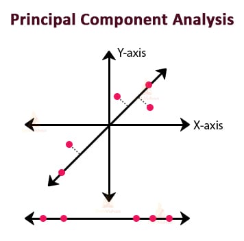

9. Neural Networks

Neural Networks are also known as Artificial Neural Networks.

Let us understand this by an example.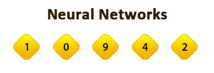

Identifying the digits written in the above image is a very easy task for humans. This is because our brain contains millions of neurons that perform complex calculations for identifying any visual easily in no time.

But for machines, this is a very difficult task to do.

Neural networks solve this problem by training the machine with a large number of examples. By this, the machine automatically learns from the data for recognizing various digits.

Thus we can say that Neural Networks are the Data Science algorithms that work to make the machine identify the various patterns in the same way as a human brain does.

10. Random Forests

Random Forests overcomes the overfitting problem of decision trees and helps in solving both classification and regression problems. It works on the principle of Ensemble learning.

The Ensemble learning methods believe that a large number of weak learners can work together for giving high accuracy predictions.

Random Forests work in a much similar way. It considers the prediction of a large number of individual decision trees for giving the final outcome. It calculates the number of votes of predictions of different decision trees and the prediction with the largest number of votes becomes the prediction of the model.

Let us understand this by an example.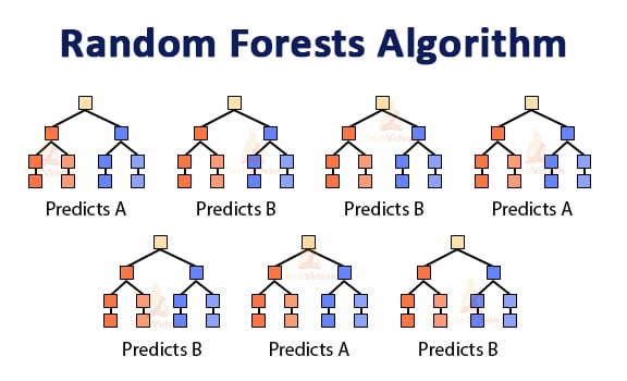

In the above image, there are two classes labeled as A and B. In this random forest consisting of 7 decision trees, 3 have voted for class A and 4 voted for class B. As class B has received the maximum votes thus the model’s prediction will be class B.

Summary

In this article, we have gone through a basic introduction of some of the most popular Data Science algorithms among Data Scientists.

There are various Data Science tools also which help Data Scientists to handle and analyze large amounts of data. These Data Science tools and algorithms help them to solve various Data Science problems for making better strategies.