Statistics for Machine Learning
Learning the mathematics of machine learning is the primary aspect to start your ML learning expedition. We often see students and other beginners facing problems when it comes to creating or understanding ML algorithms.
Well, many times the case is that they might not understand the code or also in many cases, they are not able to create the proper math formula to place in the model. This is extremely important, as the math formula not only defines your algorithm; it also decides how your model will function.
Mathematics is an all-rounder in computer science. Even outside ML, it has significance in data structures, database management, etc. It is the basis for designing any type of algorithm in computer science.
For this article, we will discuss the math involved in the fields of ML and also data science. This article will focus on both statistics and mathematics for Machine Learning.
Mathematics in Machine Learning
We will discuss the concepts of ML mathematics alongside looking at what library to import in coding and how to use it in programming. There are a multitude of concepts and some might not have a library, but a direct use in the algorithms in an expression form.
So let’s discuss these one-by-one:
1. Linear Algebra in Machine Learning
Concepts in mathematics are often used among each other. Linear algebra here is the stepping-stone to learning other concepts in ML mathematics. It covers all the necessary and basic concepts, which further have a role in other major parts of mathematics.
For the general technical definition, we can say that linear algebra is the form of representing data in an equation-like format, which we further represent in matrix and vector formats.
Linear algebra is the tool to deal with various coordinates and especially higher dimensions and planes. Also, keep in mind that not the entire concept of linear algebra comes into the picture. We only look at the concepts that help in creating models and algorithms.
For starters, you should practice solving systems of linear equations. That way you would learn how to write and solve linear equations with multiple variables.
The equations will be like:
Ax + By + Cz = d or 2x + 3y + 5z = 3
There will be two or three equations like these. We can solve them with basic cross-multiplication or elimination methods. Now comes matrices.
For matrices, learn how to write data and equations in matrix form. If you can do that, the next is only basic scalar and vector operations, which you can perfect through a bit of practice.
We have the basic arithmetic operations like addition, subtraction, multiplication and division. Learners should know these just basic arithmetic operations.
Note:- For using matrices and other math concepts in coding, we can use the NumPy library.
Also, the types of matrix products are crucial. Like, matrix-matrix, matrix-vector, and matrix-scalar products. In matrix-matrix, we just normally multiply both matrices. In matrix-vector however, we use the dot() function that comes with NumPy.
Here, the result will always be a vector.
Also, keep in mind that the matrix should have the same number of rows as the vector.
C = A.dot(B)
For matrix-scalar, a scalar quantity (number) is multiplied with each element of the matrix.
Matrix Factorization or decomposition is also there. This concept comes in handy when we have complex matrices that are hard for the algorithm to calculate.
Using decomposition, we simply reduce the matrix into smaller quantities to ease calculation.
Matrix Decomposition Methods
We have three methods for this:
– LU decomposition method
– QR decomposition method
– Cholesky decomposition method
In LU decomposition, We have the lower and upper triangular matrices. L and U here mean lower and upper.
We use a variant of LU decomposition that is the LUP decomposition where P is a type of result permuting matrix used to alter to give the same result.
It comes as a very useful method when we want to calculate the inverse of a matrix, determinants and to find values of unknown variables in equations.
A = P.L.U
Note:- LU is only for square matrices.
QR decomposition handles m*n matrices and also square matrices. Here, Q is a square matrix and R is an upper triangular matrix (m*n).
The only difference between LU and QR is that QR can handle m*n matrices.
A = Q.R
Cholesky decomposition is much more efficient than LU and QR decomposition methods.
In this, we use positive definite matrices that are also symmetric in nature (Symmetric matrices are actually transposed of themselves).
This method is helpful in linear regression and various other optimization techniques. Its shown as:
A = L.LT
We can import these using NumPy. For using them as functions, we can use:
– Scipy.linalg.lu()
– Numpy.linalg.qr()
– Numpy.linalg.cholesky()
In the matrix, one should also learn about eigenvalues and eigenvectors.
We have another crucial concept of vector calculus that covers all aspects of vectors, their operations, and their use in modern ML concepts like gradient descent and other gradient functions.
We further use this in various higher-order derivatives and differential calculus.
Note:- Vector is a matrix but with only one column and n rows.
Last but not least we have probability and distributions. Probability is an inseparable ML and data science concept and is used in creating prediction and probability-based algorithms.
First, get well versed with the basics of probability and then use it alongside other statistical methods. The related concepts in ML include the naïve Bayes classifier and the Gaussian distribution model.
Various Applications of Linear Algebra in ML
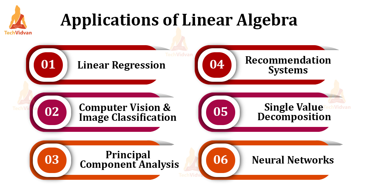
a. Linear Regression
We use this concept to determine the relationship between data and variables. It’s mainly used for predicting simple numerical values. The general way to solve this problem includes the matrix decomposition methods that we discussed above.
b. Computer Vision and Image classification
Linear algebra helps in image classification, especially in storing the information about every single image. The matrices will store the image pixels and their dimensions. We can do tasks like photo-editing using the above linear algebra concepts.
c. Principal Component Analysis
It is a dimensionality reduction method. Here, the algorithm will remove any irrelevant data by removing certain columns. This is a very robust reduction method and can be used with any algorithm.
d. Recommendation systems
Linear algebra helps to connect user preferences and results. We can use the decomposition methods here for further dimensionality reduction so as to improve the search results.
e. Single Value Decomposition
It’s another type of matrix decomposition method that helps in data visualization, feature selection, removal of unnecessary data like background noise. This can also come handy in image segregation.
f. Neural Networks
TensorFlow and other powerful libraries would encapsulate the concepts of matrices and vectors. In neural networks, linear algebra helps in higher dimensional computations. Here, linear algebra comes in algorithms of speech and text recognition, recurrent neural networks, etc.
2. Calculus in Machine Learning
There is not any deep concept to discuss regarding calculus. We have two types. Differential and Integral calculus.
Calculus helps in various deep learning and neural network algorithms. It helps in designing forward and backward propagation of any neural network. We can design certain error and loss functions using calculus.
Differentiation helps in optimization techniques and is used to find maxima and minima of functions.
Whereas, integration helps in various probability-based functions and to also calculate areas in complex mathematical graphs. Both linear algebra and calculus were the two most necessary math concepts that an ML or data science practitioner should know about.
Now comes a different part of ML mathematics that comes under the data interpretation and calculation part. Yes, we will now discuss some concepts on ML statistics.
Statistics in Machine Learning
Statistics, just like any other math concept, plays a very important role in ML. Although ML and statistics are not directly related, they come in handy for the same set of problems.
We have various areas in AI and ML, like speech recognition, pattern recognition, etc. Both ML and statistics-based algorithms aim for the same result, but they achieve it in different ways.
Basically, statistics and ML are trying to achieve the same end result, but they have very different approaches to solve problems.
ML is a branch of computer science whereas statistics belong to the math family.
Here, we have used these two individual aspects together to form various prediction based algorithms and models. Now, we will discuss the basic math in statistics that the learners should look out for.
Statistics involves a lot of working with data. It provides great tools that work on raw data and sends very precise information.
Type of Data in Machine Learning
For starters, we should know about the types of data. These are:
- Numerical
- Categorical
- Ordinal
a. Numerical Data
Numerical data means quantifiable data. Discreteness of data is very much possible as counting of some finite events can happen. The data can also behave continuously. This means it can go up to infinity as well.
For example, we can give values to parameters like height, weight, length etc.
b. Categorical Data
Categorical data doesn’t have any inherited meaning i.e., they do not show any numerical significance. So, we cannot perform any arithmetic operations on categorical data unlike in numerical data. Also, categorical data includes bar graphs and pie-charts. Unlike numerical data, they don’t have any logical order. We cannot give any value to them.
Like for example, if we say red is greater than blue, it would make no sense.

This is the image of a pie-chart. It has no numerical significance. But, it carries information.
c. Ordinal Data
Well, ordinal data comes as a type of categorical data but with a numerical scale along with it.
For example, if we say from 1 to 10, the food is a level 8 spicy. Spicy is a categorical data, we added a numerical scale to it.
So, before diving into the main agenda, let’s understand some basic statistical concepts:
Measures of Centre in ML
We use this to find the central part of the data:
1. Mean:
This is the arithmetic average. We first add all the elements of the dataset and then divide the sum with the total number of elements in the dataset.
2. Median:
Median is the middle value. We have two different cases here : for odd and even number of elements in a dataset.
For an odd number, the exact middle element in a dataset is the median. For an even number, the average of the middle two elements is the median.
3. Mode:
Mode is the most repetitive data in the dataset.
For example, in a dataset {1, 1, 1, 2, 3, 4, 5}, 1 is the mode as it’s repeating the most.
4. Mid-range:
This is the mean of the maximum and minimum values of a dataset.
For example, if we have a dataset like {1,2,3,4,5}, the mean of 1 and 5 is the mid-range of the dataset.
Measures of Variability in ML
Here, we calculate the amount of spread and dispersion in a dataset:
1. Range:
In simple terms, this is nothing but the difference between the maximum and the minimum values of a dataset. We cannot determine how centralized the data is, using range.
2. Variance:
We use it to determine how much scattering has happened in the data. More the variance, more the scattering. It’s also termed as the average of squared differences.
The reason is that, we subtract and square the difference between the value of one single observation and the mean of the dataset. After that, we take the average.
The formula is:
?2 = ∑(x – ?)2/ N
Here, x means the value of one observation. Mu is the mean and N is the number of observations. We can also take (n-1) for sample variance.
3. Standard Deviation:
It shows by how much the group elements differ from the actual mean of the group. Also, the square root of variance is the actual standard deviation.
SD = √?2
The lower the SD, the narrower the peak of the bell-curve becomes as the data is more close to the mean of the data.
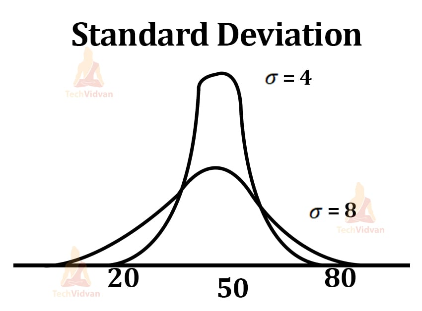
This is a rough diagram, but the real-thing looks closely appropriate.
Measures of Position in ML
It’s used to measure the position of a particular data value in a given dataset.
1. Percentile:
It is a measure in statistics under which a certain percentage of data comes under.
For example, in a group of 10, Ajay is the third tallest guy. So, Ajay here is the third percentile and the rest of the 70 odd percent of people fall shorter than Ajay.
To calculate percentile, we should sort the data first.
2. Z-score:
Z-score tells us by how many standard deviations a particular data comes above or below the mean. If the value comes out as positive, then the value is above average. If not, it’s below average.
Z = (x – ?)/?
3. Quartile:
A quartile divides the dataset into three or more than three equal parts.
For four equal parts, we divide the data points as, the minimum, the 25th percentile, the 50th percentile, the 75th percentile and the maximum.
Here the 25th percentile is the Quartile 1 or Q1. And 75th percentile is the Q3.
The 50th percentile is the median. From this, we get a new term the Inter-Quartile Range (IQR).
IQR = Q3 – Q1
We have two types of statistics in knowledge:
- Descriptive Statistics
- Inferential Statistics
1. Descriptive Statistics
It helps in the description and summarization of data. It includes both numerical and graphical representation methods.
We have two special concepts under this:
- Here, we face the basic concepts of mean, median, and mode. These can calculate average, mid-value, and most repeated values.
- Collectively, they are the measure of central tendency.
- Here, we describe how much spread the data is. In this, we discuss concepts like standard deviation, quartiles, variance, etc.
- The concept is about the dispersion of data.
- For example, if the mean score of a school is 50, it does not mean that all students have scored well. Some will have very good marks and some will have very bad.
- The data is quite spread out in this manner. Collectively, these come under the measure of spread.
- We also have terms like skewness of data to look if the accumulated data falls either towards the left or right side in the graph.
- Kurtosis is also a concept where we analyze the extremities of the dataset. And then we have variability to measure the distance between data points and central mean area.
- We can measure variability using the range, variance, standard deviation, etc.
2. Inferential Statistics
It takes samples from a large population and draws an estimate or an assumption that would represent the entire population.
For example, in quality testing, the whole bunch of products is not tested for quality, but we take a sample for small batch testing.
Similarly, we can’t find the marks of students of an entire country. But we can take a small data of students and then draw an assumption from it.
In short, we can draw inferences for data that is either not known or inaccessible. The process of taking samples from large populations is what sampling is.
Techniques for Inferential Statistics in Machine Learning
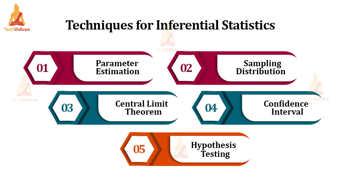
Parameter estimation:
The parameters used for selecting the best dataset and to draw an accurate generalization need careful choosing, as chances of error loom over.
Sampling Distribution:
In sampling distribution, we visualize the sampling means data in the form of a curve. It doesn’t exactly represent how the population would look. Because the graph can be of any curved shape for any population. The shape of the graph never changes (curved-bell).
Central Limit Theorem:
We studied that Sampling distribution shows us how the population would look. Now, CLT will show us how it’s possible. Here, the means of sample and that of the population are the same. Also, the normal distribution for the sampling distribution will be σ/√n.
Sigma is the standard deviation and n is the sample space.
An important point to note, the population distribution shape will not affect the shape of the sampling distribution (curved-bell). The more the size of the sample, the lesser chances of error occurrence.
Confidence Interval:
The interval in the sampling distribution curve within which most of the sample data comes.
Hypothesis Testing:
In hypothesis testing, we generate a lot of assumptions. We compare the sample stats with that of the population or we can use a different example to analyze any interventions.
We have two types of hypotheses. Null and Alternate Hypothesis.
In the Null hypothesis, we assume the sample and population stats to be the same. For example, a previous result would be the same as the result.
But in an Alternate hypothesis, we assume that both results are different. It is like a contradiction of the null hypothesis.
So, these were the concepts of statistics of ML and data science.
Conclusion
Finally in this article, we have covered various small and important concepts of Statistics for Machine Learning.
Next we have studied how to use them in coding format. Please remember that it is absolutely necessary for anyone to know these concepts for pursuing ML or data science. These concepts are the backbone of all the algorithms and models that we design. The research field is many times about creating better models.