SVM in Machine Learning – An exclusive guide on SVM algorithms
Support Vector Machine is a classifier algorithm, that is, it is a classification-based technique. It is very useful if the data size is less. This algorithm is not effective for large sets of data. For large datasets, we have random forests and other algorithms.
Learning this is very important as it is both useful in making models, but also it is the base for other concepts. By learning about SVM in Machine Learning, we can learn other algorithms like gradient descent, etc.
In this article, we will be learning various things about the SVM. We will look at code samples to understand the algorithm. Also, we will be studying about libraries with which we can design an SVM and many more things.
So let us begin.
What is SVM in Machine Learning?
An SVM is a classification based method or algorithm. There are some cases where we can use it for regression. However, there are rare cases of use in unsupervised learning as well.
SVM in clustering is under research for the unsupervised learning aspect. Here, we use unlabeled data for SVM. Since the topic is under research, we will only look at what it means.
In regression, we call the concept SVR or support vector regression. It is quite similar to SVM with only a few changes. However, it is more complicated than SVM.
Now, we come to SVM. It is a strong data classifier.
The support vector machine uses two or more labelled classes of data. It separates two different classes of data by a hyperplane. The data points based on their position according to the hyperplane will be put in separate classes.
In addition, an important thing to note is that SVM in Machine Learning always uses graphs to plot the data. Therefore, we will be seeing some graphs in the article.
Now, let’s learn some more stuff.
Parts of SVM in Machine Learning
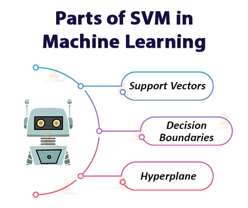
To understand SVM mathematically, we have to keep in mind a few important terms. These terms will always come whenever you use the SVM algorithm. So let’s start looking at them one by one.
1. Support Vectors
Support vectors are special data points in the dataset. They are responsible for the construction of the hyperplane and are the closest points to the hyperplane. If these points were removed, the position of the hyperplane would be altered. The hyperplane has decision boundaries around it.
The support vectors help in decreasing and increasing the size of the boundaries. They are the main components in making an SVM.
We can see the picture for this.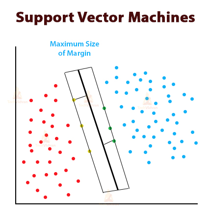
The yellow and green points here are the support vectors. Red and blue dots are separate classes.
The middle dark line is the hyperplane in 2-D and the two lines alongside the hyperplane are the decision boundaries. They collectively form the decision surface.
2. Decision Boundaries
According to the SVM algorithm we discover the points closest to the road from both the classes. These points are called support vectors. Decision boundaries in SVM are the two lines that we see alongside the hyperplane.
The distance between the two light-toned lines is called the margin. An optimal or best hyperplane form when the margin size is maximum. The SVM algorithm adjusts the hyperplane and its margins according to the support vectors.
3. Hyperplane
The hyperplane is the central line in the diagram above. In this case, the hyperplane is a line because the dimension is 2-D. If we had a 3-D plane, the hyperplane would have been a 2-D plane itself. There is a lot of mathematics involved in studying the hyperplane.
We will be looking at that. But, to understand a hyperplane we need to imagine it first.
Imagine there is a feature space (a blank piece of paper). Now, imagine a line cutting through it from the center. That is the hyperplane.
The math equation for the hyperplane is a linear equation.
a0 + a1x1 + a2x2 + ……. + anxn
This is the equation.
Here a0 is the intercept of the hyperplane. Also, a1 and a2 define the first and second axes respectively. X1 and X2 are for two dimensions.
Let us assume that the equation is equal to E. So if the data points lie beneath the hyperplane then E<0. If they are above it, the E>=0. This is how we classify data using a hyperplane.
In any ML method, we would have the training and testing data. So here we have n*p matrix which has n observations and p dimensions.
We have a variable Y, which decides in which class the points would lie. So, we have two values 1 and -1. Y can only be these two values in any case.
If Y is 1 then data is in class 1. If Y is -1 then data is in class -1.
Based on all this information, we have a small code here. This code will perfectly explain the conditions above.
import numpy as np
from matplotlib import pyplot as plt
We will use only basic libraries for now, as it is only an example. Here we are using NumPy for math operations on the array of data.
Also, we are using matplotlib for plotting the graph.
a = np.array([[0,3,-1],
              [2,2,-1],
              [2, 5, -1],
              [2, 4, -1],
              [4, 5, -1]
             ])

b = np.array([-1,-1,1,1,1])

for i, sample in enumerate(a):
    if i < 2:
        plt.scatter(sample[0], sample[1], s=150, marker='*', linewidths=3)
else:
        plt.scatter(sample[0], sample[1], s=150, marker='o', linewidths=3)

plt.plot([-2,6],[5,1.5])
Here we have ‘a’ variable that holds the array of data. This data is the coordinates of the points on the dataset. Here, ‘b’ is the data specifying in which class the points lie.
The program plots the data as ‘*’ for one class and ‘o’ for another. Based on the ‘if’ condition it places the datapoints above or below the hyperplane.
The sample data helps the algorithm to plot the data. ‘s’ is the length of the hyperplane. Linewidth is the thickness of the hyperplane.
All of this data runs in a ‘for’ loop which takes in data from ‘a’.
The last line of code plots the hyperplane. The coordinates of the plot function are the coordinates of the two end-points of the hyperplane.
The result of this code in graphical format is shown below.
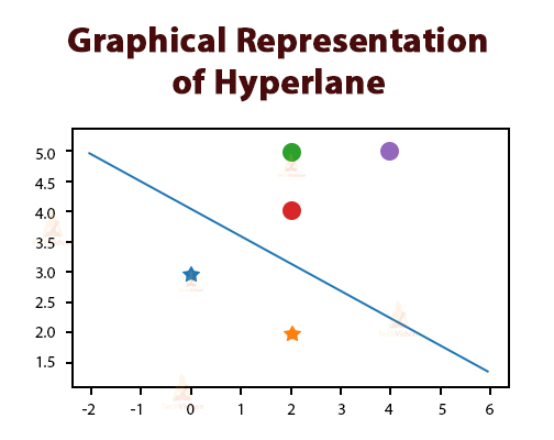
The hyperplane has many concepts like the maximum margin classifier that is used in setting the maximum margin of the plane. The maximum margin classifier helps to adjust the hyperplane and the decision boundaries.
Still, there can be cases where data can be indistinguishable and hence, where we cannot draw a hyperplane.
Here, we could use quadratic or cubic equations to define the problem. The concept used here is the support vector classifier. Here, we try to solve things by increasing the size of feature space by using kernel tricks and all that.
Kernel trick is the inner product of two support vectors that increases the size of the feature space.
We increase the feature space for displaying the non-linear equation results, which can be curves and all. This is all for data which is inseparable and to which hyperplane is not possible.
This was all about the hyperplane.
At last, we can discuss where we can use SVM in Machine Learning. It can be used in places like image classification. We can use it in biometrics. It can be used to design security codes. We can use it for protein classification and there are many more uses to it.
How Does an SVM Work?
For this, let us compare the working of SVM and other classifiers for better understanding. Let us talk about SVMs and perceptrons.
Perceptrons and other classifiers focus on all the points that are present in the data. For these classifiers, the focus is more on just separating the complex points and adjusting the dividing line.
Perceptrons are made by taking one point at a time and fixing the dividing line accordingly. When all the complex points are separated, the perceptron algorithm stops.
This is the end of the process for these classifiers, as they do not improve the position of the dividing line. So, finding the optimal dividing line is not what the perceptron does.
Whereas, the case with SVM is a little different. In this, the algorithm only focuses on the points that are complex to separate and it ignores the rest of the points.
The algorithm finds the points that are closest to each other. It then draws a line between them. The dividing line would be optimal if it is perpendicular to the line connecting the points. The best part is that two different classes are formed on either side of the line. Whatever new point enters the dataset, it won’t be affecting the hyperplane.
The only points that would affect the hyperplane are the support vectors. The hyperplane won’t allow the data from both classes to mix in most cases.
Also, the hyperplane can adjust itself by maximizing the size of its margin. The margin is the space between the hyperplane and the decision boundaries.
This is how the SVM in Machine Learning works.
Implementation of SVM in Python
Machine Learning as we know can be programmed with various languages and Python is one of them. We generally prefer Python as it is relatively easier to code with than other languages like Java. Now let’s look at how it is implemented in Python.
SVM in Machine Learning can be programmed using specific libraries like Scikit-learn. We can also use simpler libraries like pandas, NumPy, and matplotlib. We can understand this with some codes.
Note: If you are doing this on Google colab, you need to first upload the dataset from your drive to Google colab. This is shown in the link below.
Dataset: Implementation of SVM in Python
1. First, we import the libraries.
import pandas as pd
import numpy as np
import matplotlib.pyplot as plt
2. Now, we import datasets.
data = pd.read_csv('creditcard.csv')
3. After importing the data, we can view the data by applying some basic operations.
In this step, we explore the data and analyze it.
data.head()
This is the output of data analysis.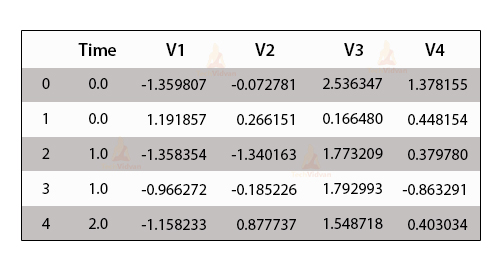
4. The next step is a very crucial step in SVM in Machine Learning. Here, we perform Data Preprocessing. This step divides the data into attributes and labels data.
5. In preprocessing, we divide the attributes and labels into two variables. Here, we take a particular column from the data. The column is dropped from the first variable. The second variable now holds the dropped column.
X = data.drop('Class', axis=1)
y = data['Class']
6. Now, after the data gets separated into attributes and labels, we arrive at the final preprocessing step. Now, we use the Scikit-learn library for dividing data into training and testing data.
from sklearn.model_selection import train_test_split
X_train, X_test, y_train, y_test = train_test_split(X, y, test_size = 0.20)
7. The above step shows that the train_test_split method is a part of the model_selection library in Scikit-learn. Using this, we will divide the data. When we run this command, the data gets divided.
8. Now, the next step is training your algorithm.
from sklearn.svm import SVC
svclassifier = SVC(kernel='linear')
svclassifier.fit(X_train, y_train)
9. The training of data is done by using the SVM library. This library has built-in functions and classes for various SVM algorithms. We also use a library for classification. This library is SVC or support vector classifier class. We have to specify the type of kernel we are using in this class.
The code snippet is mentioned above, whereas the image of the output of this snippet is given below.
10. The fit method of the SVC class used above trains the algorithm.
11. After training, we use the predict method to give predictions.
y_pred = svclassifier.predict(X_test)
12. The last step is evaluating the algorithm and finding the result for the SVM.
from sklearn.metrics import classification_report, confusion_matrix
print(confusion_matrix(y_test,y_pred))
print(classification_report(y_test,y_pred))
This is the output that is given in image format.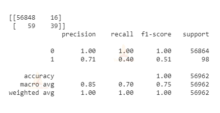
13. This code does not include plotting graphs. We have just seen an example of how to train and test the data. Also, we saw how to train the algorithm.
14. This sums up the implementation of SVM using Python language.
How to Tune SVM Parameters?
SVM parameters improve the quality of the hyperplane and are inserted as normal parameters in the Python code. These parameters determine the shape of the hyperplane, the transition of data between decision boundaries, etc.
There are overall four main types of parameters that we should know. These are:
- Kernel Parameters
- Gamma Parameters
- C Parameters
- Degree Parameters
Let’s discuss each of them in detail.
Kernel Parameters
In Kernel parameters, also we have four types which are linear, RBF, polynomial and sigmoid. The kernel parameters determine the shape and structure of the hyperplane. By tuning, we can set the kernel type and the model adapts to it.
Gamma Parameters
The gamma parameter is for non-linear hyperplanes. Here, the kernel value is RBF, polynomial or sigmoid. This parameter tries to fit in all the data.
C Parameters
The C parameter is more like a penalty parameter. It tells us that if the value of C is high then, the datapoints further away from the plane are also important to us. This makes us include them also and this leads to overfitting.
Degree Parameters
Finally, the degree parameter. This parameter uses ‘poly’ as the kernel value. The degree parameter helps to find the hyperplane for splitting data. Then the degree of the polynomial helps in this. The more the degree of polynomial increases, the more training time it takes. By tuning all these values, one can control the hyperplane as well as the model of SVM.
Pros and Cons of SVM in Machine Learning
Now, let’s discuss the advantages and disadvantages of SVM in Machine Learning.
Pros of SVM in Machine Learning
- SVMs have better results in production than ANNs do.
- They can efficiently handle higher dimensional and linearly inseparable data. They are quite memory efficient.
- Complex problems can be solved using kernel functions in the SVM. This comes under the kernel trick which is a big asset for SVM.
- SVM works well with all three types of data (structured, semi-structured and unstructured).
- Over-fitting is a problem avoided by SVM. This is because SVM has regularization parameters and generalization in its models.
- There are various types of kernel functions for various decision functions.
- We can add different kernel functions together to achieve more complex hyperplanes.
Cons of SVM in Machine Learning
- Choosing a kernel function is not an easy task (especially a good one).
- The tuning of SVM parameters is not easy. Their effect on the model is hard to see.
- SVM takes a lot of time for training with large datasets.
- It is hard to predict the final model as there can be a lot of minute changes. So, recalibrating the model each time is not a solution.
- If there are more features than samples in the data, the model will give a poor performance.
Summary
In this article, we looked at many aspects and uses of the SVM in Machine Learning. We first understood what the algorithm signifies. Then we analyzed the terminologies involved in the algorithm. We looked at mathematical equations that define the SVM.
Also, we even looked at a piece of code that gives a basic understanding of SVM in Machine Learning. We learned how to tune SVM parameters and saw another implementation and code snippets in Python.
Then, we studied how the SVM works and what are their advantages and disadvantages. Finally, we looked at some uses of SVM in real life which are many, but we looked at the important ones.
This would be all for SVM in Machine Learning.