Tree in Data Structure
What is a Tree Data Structure?
A tree is a non-linear data structure. In a tree, data is stored in the hierarchical form at multiple levels. This data is stored in nodes. The nodes are linked together to each other based on their hierarchy. Each node contains two things: a data value and a pointer to link to other nodes.
Why use Tree Data Structure?
Whenever we have large amounts of data, the operations on linear data structures become costly and have more complexity. In such cases, non-linear data structures like trees save the time to compute a particular operation. We can reduce their cost for some operations, by using non-linear data structures instead of linear data structures.
Tree Terminologies:
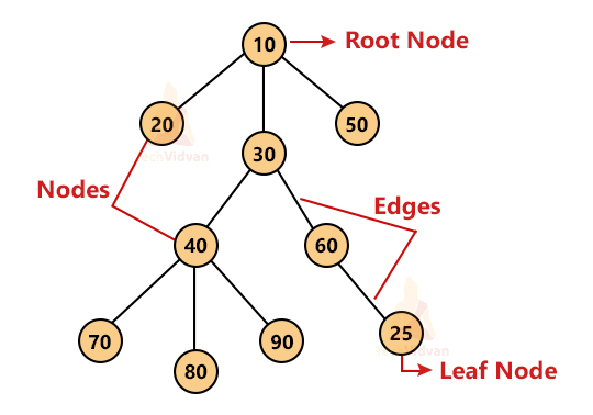
Consider the following tree:
1. Node: A node contains the data value and the pointers to other nodes. Here, 10, 20, 30, 50, 40, 60, 70, 80, 90 and 25 are the nodes.
2. Edge: The line that links any two nodes is termed the edge.
3. Child node: It is the node immediately below a particular node. It is the child/descendent in the hierarchy. For example, 70, 80 and 90 are the child nodes of 40.
4. Parent node: It is the node immediately above a node. It is the ascendant in the hierarchy. For example, 40 is the parent node of 70, 80 and 90.
5. Root node: A node having no parent node is the root node. It is the topmost node of the tree. Here, 10 is the root node.
6. Leaf node: A leaf node is the one having zero children. It is the bottom-most node in the tree. In the above example, we have 6 leaf nodes: 20, 50, 70, 80, 90 and 25.
7. Internal node: Nodes with at least one child are the internal nodes. For example, 30 and 40 are internal nodes.
8. Ancestor: If there are two nodes, say P and Q and there is a path from P to Q, then P is the ancestor of Q. For example, in the above tree, 10 is the ancestor of 50, 70.
9. Descendent: It is the opposite of an ancestor. For example, 70 is the descendent of 30.
10. Sibling: Two nodes having the same parent are known as siblings. For example, 70, 80 and 90 are siblings.
11. Generation: Nodes at the same level of the tree are termed as a generation. For example, 70, 80, 90 and 25 belong to the same generation.
Properties of Tree Data Structure:
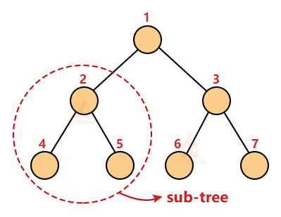
1. Recursive Data structure: Recursive data structures are those which derive themselves from their structure. A tree has multiple sub-trees associated recursively with it. Every sub-tree has its won root node and children nodes.
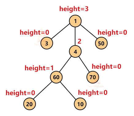
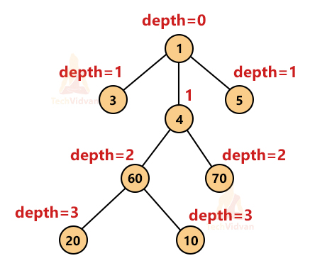
2. Height of a node: Height is the length of the path from a particular node to the farthest leaf node. Height is always measured from bottom to top. Thus, the height of each leaf node is 0. The following diagram shows the height of different nodes:
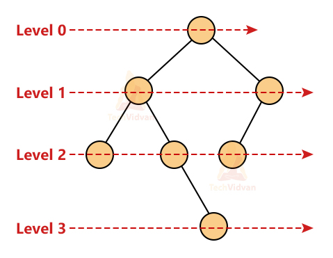
3. Level of a node: Level is measured with respect to the root node. The level is defined as a step from top to bottom.
4. Depth of a node: It is the reverse of height. The depth of the root node is zero. The depth of any other node is the number of edges it has from the root node.
5. Number of edges: In a tree having n nodes, the number of edges will be n-1. Except for the root node, every other node in the tree will have at least one incoming edge.
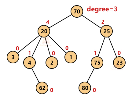
6. Degree of a node: The degree of any node tells the number of children of that node. Thus, leaf nodes have degree zero.
7. Degree of a tree: The degree of a tree is the maximum of all the possible degrees of its nodes. For example, the degree of the above tree is 4.
Types of Trees in Data Structure
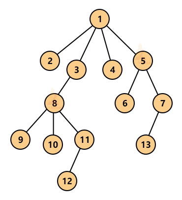
1. General tree: A general tree can have any degree. It has no restriction on how many children nodes a given parent node can have. The following diagram shows a general tree:
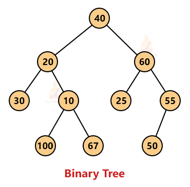
2. Binary tree: A binary tree is one that can have a maximum of only 2 children nodes. The node of a binary tree consists of three things- a data item, a pointer to the left child and a pointer to the right child. There are various types of binary trees such as a full binary tree, complete binary tree, perfect binary tree, skewed binary tree, etc.
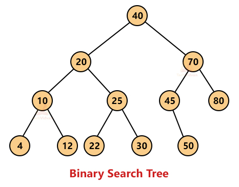
3. Binary search tree: A binary search tree is a special type of binary tree in which the left child is always smaller than the parent node and the right child is always greater than the parent node.
4. AVL tree: An AVL tree is a height-balanced binary tree. In an AVL tree, the difference between the height of the left sub-tree and the height of the right sub-tree is either 0, 1 or -1. This difference is termed the balancing factor.
An AVL tree is more efficient in terms of complexity as compared to a simple binary tree because of its balancing property. The following tree is an AVL tree:
5. Red-black tree: A red-black tree is a self-balancing binary search tree. A red-black tree balances itself in two rotations whereas an AVL tree could take any number of rotations for balancing. In a red-black tree, each node is labelled as either red or black and an extra bit is used to store this information for each node. A red-black tree is also more efficient than a simple binary search tree because of its balancing properties.
6. Splay tree: It is also a self-balancing binary tree. In the splay tree, the most recently accessed node becomes the root node by performing some rotations. The term splaying is used for the most recently accessed node. A splay tree is a balanced tree but it might not be height-balanced. The splay tree takes O(log n) time for performing its operations.
7. Treap: It is a combination of tree and heap. It has the properties of both binary search trees and heap data structures. Every node in the treap data structure contains a key and a priority. The key comes from the binary search tree and priority comes from the heap data structure.
In a binary search tree, the data in the left child is always smaller than the root and the data in the right child node is always greater than the root. So is the case of treap. Also, in a treap, the children of any sub-tree have a greater value than the root node of that subtree(property of heap data structure).
8. B-tree: Just like binary trees have degree 2, the B-trees have a degree m, where m could be any value greater than or equal to 2. A B-tree is an m-way tree that can have more than 1 key in each node and every node can have a maximum of m children.
Tree Traversal:
Tree traversal means visiting each node of the tree. There are broadly three types of tree traversals:
1. Inorder traversal
2. Pre-order traversal
3. Post-order traversal
Memory Representation of Tree:
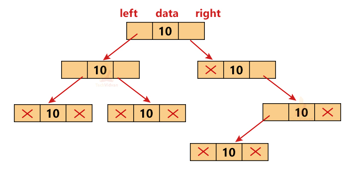
The most important component of tree data structure is a node. We can create nodes dynamically in a tree with the help of pointers. The following diagram is a memory representation of the tree data structure.
Each node contains 3 fields: a data item, a pointer to the left child and a pointer to the right child. The first and the third fields store addresses of other nodes and help to link the tree with other nodes. The second field contains the actual value of the node.
Implementation of Tree:
We can define this structure of the tree in a programming language using a heterogeneous data type such as struct as shown:
struct Node
{
    int key;
    struct Node *left_child;
    struct Node *right_child;
}
Applications of Trees:
1. Hierarchical structure: Trees follow the hierarchical structure and thus help to store data in the form of a hierarchy. For example, a file system follows a hierarchy as it is comprised of disk drives, folders, sub-folders and then files.
2. Heap: The heap data structure is another application of trees used for sorting and for implementing priority queues.
3. Binary search tree: It is an efficient form of a simple tree and is used to find whether a data item is present in a set or not.
4. Trie: Trie is another implementation of the tree data structure. It is used for storing routing information in routers as well as for storing data in the form of a dictionary.
5. B-tree and B+-tree: Both of them are used to store indexed data in databases. They are very efficient for range queries.
6. Organized data: Trees help in organizing the data more efficiently, making operations such as search, insert and delete easier to perform.
7. Routing tables: Routing tables of routers make use of trie data structure to store information.
8. Syntax tree: whenever we write our code in a programming language, the compiler makes use of the syntax tree to ensure the syntactical correctness of the code.
Conclusion
In this article, we covered one of the most important data structures i.e. tree data structure, various types of trees used in computer science and their application areas. We have also seen the implementation of these types in different programming languages. This article also covers tree traversal techniques, their implementation and their uses.

