Decision Trees in R Analytics
In this article, we are going to study decision trees in R programming and their implementation. We will learn what are R decision trees. We shall also look at how to create them and what rules govern them. Finally we will also observe their applications in the real world. So, without any distractions, let’s jump right into it.

Decision Trees in R
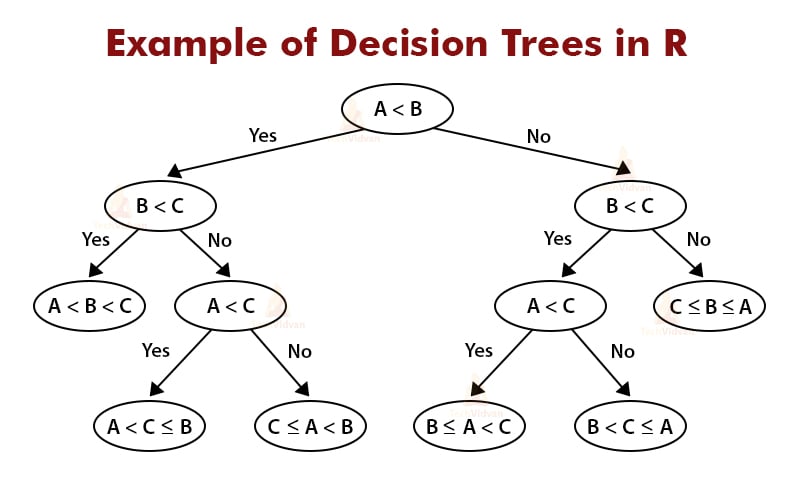
Decision trees are a graphical method to represent choices and their consequences. It is a popular data mining and machine learning technique. It is a type of supervised learning algorithm and can be used for regression as well as classification problems. Here are a few examples of decision trees.
Parts of a Decision Tree in R
Let us take a look at a decision tree and its components with an example.
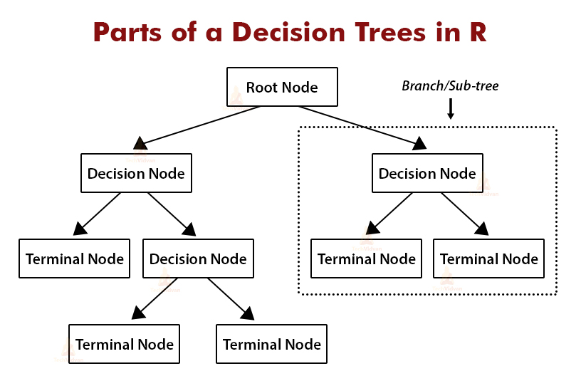
1. Root Node
The root node is the starting point or the root of the decision tree. It represents the entire population of the dataset.
2. Sub-node
All the nodes in a decision tree apart from the root node are called sub-nodes.
3. Decision nodes
When a sub-node splits and further into more sub-node. Then it is called a decision node.
4. Terminal node
Sub-nodes that exist at the ends of a decision tree are called terminal nodes or leaf nodes.
5. Branch
A branch of a decision tree also known as a sub-tree, is a subset of the decision tree. It is a part of the entire tree.
6. Child and parent nodes
When a node divides into sub-nodes, these sub-nodes are said to be the children or child nodes of that node and the original node is called the parent node.
Types of Decision Trees in R
There are two main types of decision trees. These are:
1. Regression trees in R
Regression trees are decision trees that split a dataset of continuous or quantitative variables. They are made by using the recursive binary splitting technique. As the name suggests, the recursive binary splitting technique splits the dataset into two parts repeatedly until every terminal node contains less than a specific number of observations.
Recursive binary splitting is a greedy, top-down algorithm that tries to minimize the residual sum of squares.
2. Classification trees in R
A classification tree is very similar to a regression tree except it deals with categorical or qualitative variables. In a classification tree, the splits in data are made based on questions with qualitative answers, therefore, the residual sum of squares cannot be used as a measure here. Instead, classification trees are created based on measures like classification error rate, cross-entropy, etc..
Creating a R Decision Tree
The procedure for creating a decision tree involves four important steps. These steps are as follows:
1. Choosing a variable and separation
Choosing a variable and separation criterion is largely dependent on the situation and the decision tree. In the case of a categorical output, the separation criterion is very simple. When the output is a continuous variable, the separation can have n-2 values, where n is the total number of values of the variable. The most common approach is to take the mean of all the observations of the variable.
2. Creating different nodes
There are multiple methods for forming the various nodes in the tree based on the type of output variable. One such method is the Gini test. The Gini test is a cost function that evaluates the splits in the dataset. The equation for the Gini test is as follows:

3. Splitting the data among different nodes
Once the nodes have been created, the data needs to be split among the different nodes where they fit. This process of assigning different data points to different nodes is done with the help of the decision criterion or the separation criterion decided in the first step.
4. Pruning the tree
The process of removing nodes from a decision tree is known as pruning. Pruning can also be thought of as the opposite of splitting. Once the tree has been created and the data has been assigned to it, the final step in the creation of decision trees is to prune unwanted nodes. We use cross-validation to consider which sub-trees can be removed.
Applications of Decision Trees in R
Decision trees are very useful in solving classification and regression problems. Here are a few examples of real-world applications of decision trees.
1. Medical diagnosis
Many doctors and medical researchers use decision trees formally or informally for medical diagnoses, medicinal research related inference and prediction etc.. Decision tree is the most commonly used algorithm for diagnoses by doctors all over the world. The doctors use the symptoms displayed by the patient as deciding factors to follow predetermined trees that tell whether a patient is suffering from a particular disease or not.
2. Marketing
Decision trees help in the decision-making process in the marketing sector. This helps them achieve their goals like target audience, censorship hurdles, etc.. Decision trees also help them understand the consequences of their decisions and helps them formulate their responses in the future.
3. Banking
Banks use decision trees to predict the customer they might risk losing and also to find whom to provide more and better services. This helps them in reducing their churn rates.
Practical Implementation of Decision Trees in R
Let’s look at a practical implementation of decision trees in R programming. We will be using the tree and ISLR packages and the car seats dataset for this.
1. Let us load the required packages as well as the dataset we will be using.
library(tree)
library(ISLR)
data <- Carseats

2. Let us examine the dataset that we are going to work on.
str(data)
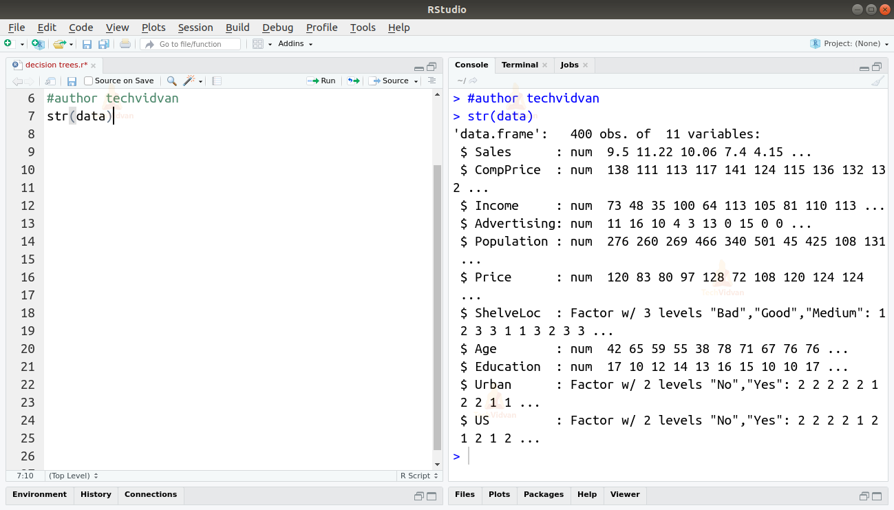
As we can see, the dataset consists of 400 observations of 11 different variables.
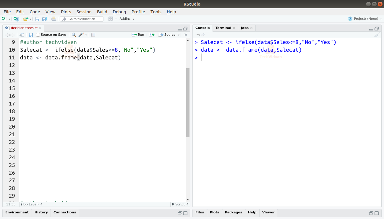
3. Sales is a variable that shows the number of sales in a particular area. It would be a suitable variable for our decision tree. But it would be much easier with a categorical variable instead of a continuous variable like Sales. Let us convert Sales into a categorical variable then.
We can introduce a new variable Salecat. The value of salecat will be Yes when Sales > 8, otherwise it will be No.
Salecat <- ifelse(data$Sales<=8,"No","Yes")
data <- data.frame(data,Salecat)
Output
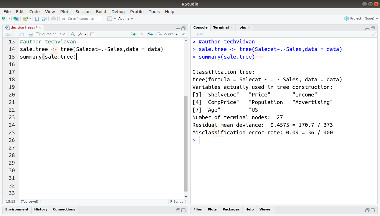
4. Now, let’s create a decision tree and fit this model. We will use the tree() function of the tree package for this. Our variable shall be Salecat and we will omit Sales form the model.
sale.tree <- tree(Salecat~.-Sales,data = data)
summary(sale.tree)
5. Let us plot the tree and see results for ourselves.
plot(sale.tree)
text(sale.tree, pretty=0)
Output

6. The result is really messy. There are too many nodes and none of them are clearly visible. A decision tree is not very efficient with this many nodes. Therefore, our next step would be to prune the unwanted nodes off this tree. To do this we will make separate training and testing datasets by drawing random samples from the original dataset.
Then we will fit the model again, this time using the training dataset in the subset argument of the tree() function.
set.seed(40)
tree.train <- sample(1:nrow(data),250)
sale.tree <- tree(Salecat~.-Sales,data,subset=tree.train)
plot(sale.tree)
text(sale.tree, pretty=0)
Output
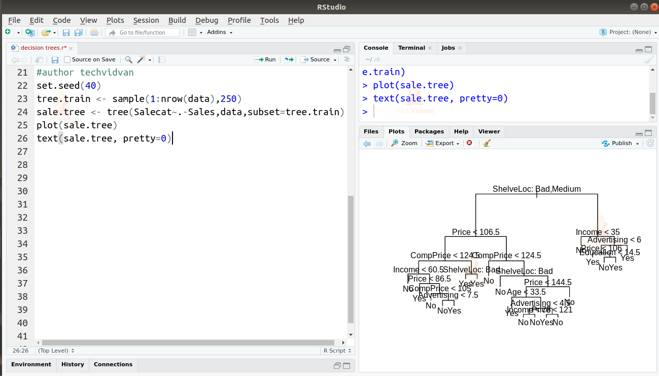
7. As the dataset is slightly different, the plot looks a bit different but the differences are not that significant. Let us now use this model to predict the results in the testing dataset. We can then compare the results with the actual Salecat variable to measure the accuracy of the model.
sale.pred = predict(sale.tree, data[-tree.train,], type="class")
with(data[-tree.train,], table(sale.pred, Salecat))
Output
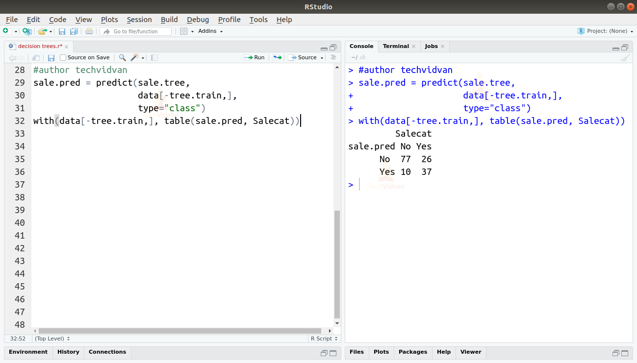
8. We can get the accuracy of the model by dividing the number of correct predictions by total number of attempts.
A=(77+37)/150=0.76
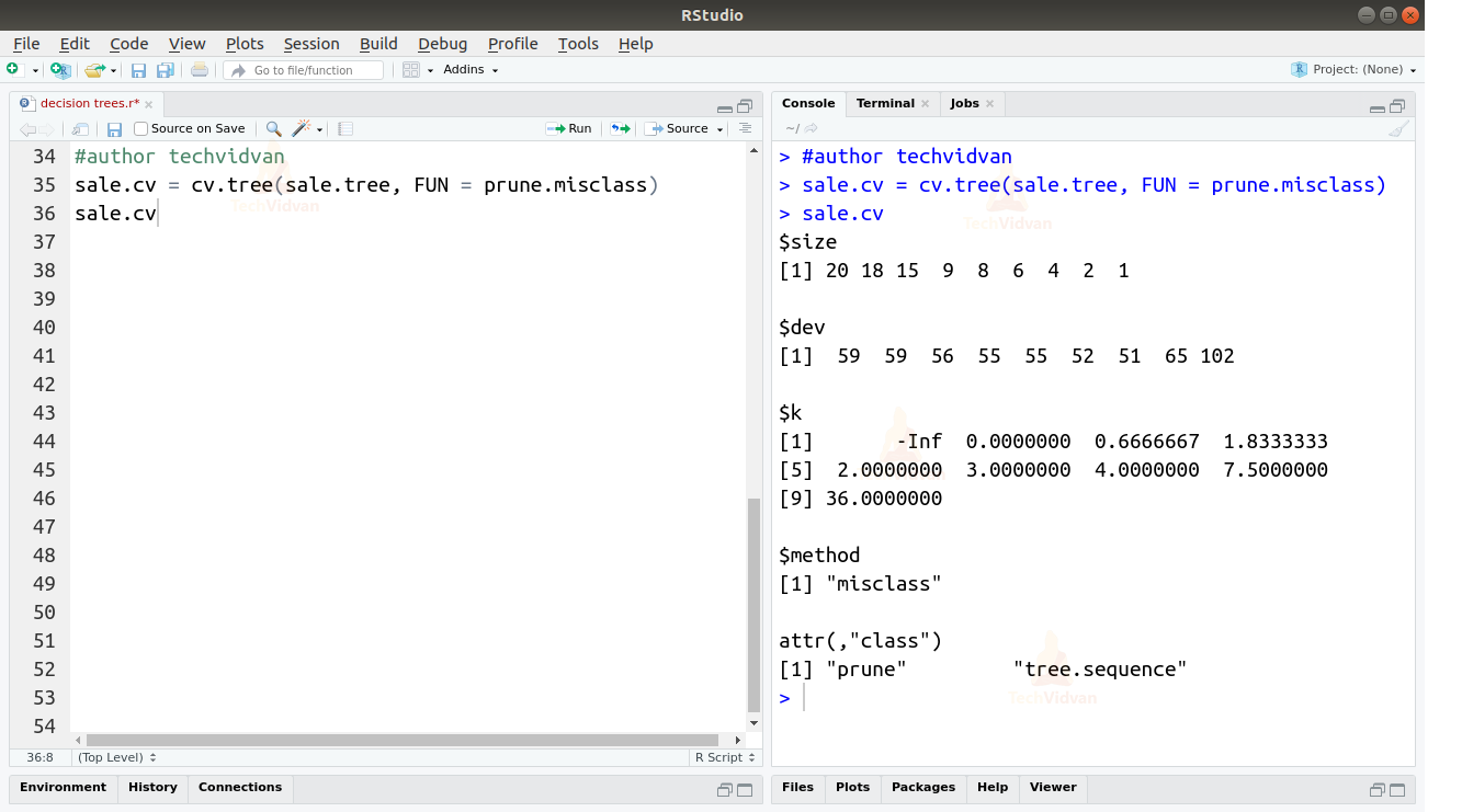
Which gives us 76% accuracy. We can use cross-validation to prune this tree more effectively. We can use the cv.tree() function for that.
sale.cv = cv.tree(sale.tree, FUN = prune.misclass)
sale.cv
Output
9. Let us now plot the cross-validation curve for this model. We will see a downward drop in the curve which will show us mismatches in the model and tell us how to prune it.
plot(sale.cv)
Output
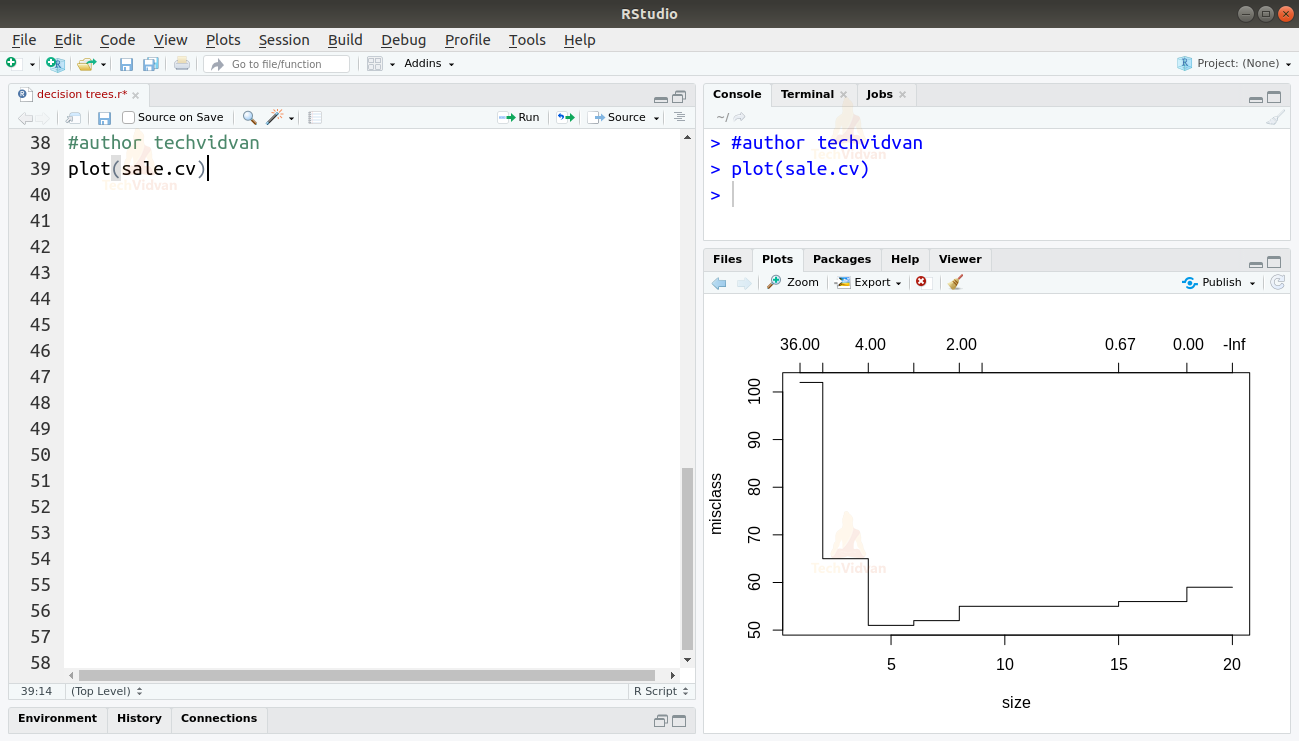
10. As the drop begins around 12, let’s prune our model to a size of 12. We can do that by using the prune.missclass() function. We will then plot the pruned tree.
sale.prune = prune.misclass(sale.tree, best = 12)
plot(sale.prune)
text(sale.prune, pretty=0)
Output
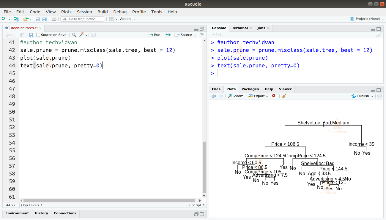
11. As we can see, the tree is now simpler and easier to understand. Let us test it again by predicting the test dataset again.
sale.pred = predict(sale.prune, data[-tree.train,], type="class")
with(data[-tree.train,], table(sale.pred, Salecat))
Output
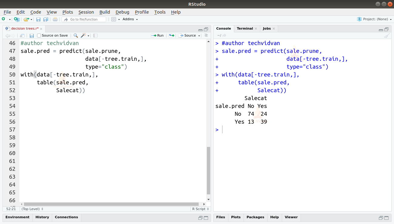
The new accuracy of the model is:
A=(74+39)/150=0.754
As we can see the accuracy has had very little effect while the tree has become much simpler. Thus, we have a model that can predict sales with reasonable accuracy.
Summary
In this chapter of the TechVidvan’s R tutorial series, we learned about decision trees in R. We studied what are decision trees and looked at the various parts of a decision tree. Then we moved on to the different types of R decision trees and learned how to create R decision tree. We also looked at the various applications of decision trees in real-life. Finally, we saw a practical implementation of decision trees in R.
Hope you enjoyed the article. Do not forget to share you rating on Facebook.