R Logistic Regression Types and Implementation

In this R tutorial, we are going to study logistic regression in R programming. We will learn what is R logistic regression. We will also look at the theory and procedure of logistic regression. Then We shall then move on to the different types of logistic regression. Finally, we will end the chapter with a practical application of logistic regression in R. So let’s get going!

Logistic Regression in R

Logistic regression is a regression model where the target variable is categorical in nature. It uses a logistic function to model binary dependent variables.

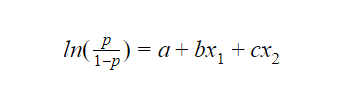
In logistic regression, the target variable has two possible values like yes/no. Imagine if we represent the target variable y taking the value of “yes” as 1 and “no” as 0. Then, according to the logistic model, the log-odds of y being 1 is a linear combination of one or more predictor variables. So let’s say that we have two predictor or independent variables namely x1 and x2, and let p be the probability of y being equal to 1. Then according to the logistic model:

By exponentiating the equation, we can recover the odds:

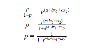
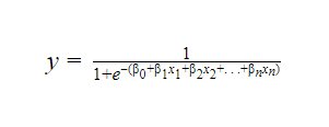
Which gives us the probability of y being 1. If p is closer to 0, then y=0 and when p is closer to 1 then y=1. Thus the equation for logistic regression becomes:

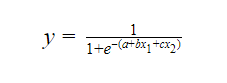
We can generalize this equation for n number of parameters and independent variables as follows:

Types of R Logistic Regression

There are three types of logistic regressions in R. These classifications have been made based on the number of values the dependent variable can take.

1. Binary logistic regression in R

In binary logistic regression, the target variable or the dependent variable is binary in nature i.e. it has only two possible values.

Ex: whether a message is a spam message or not.

2. Multinomial logistic regression

The target variable in a multinomial logistic regression can take three or more values but these values do not have any definite order of preference.

Ex: the most preferred type of food (Indian, Italian, Chinese, etc.)

3. Ordinal logistic regression

In ordinal logistic regression, the target variable has three or more possible values and these values have an order or preference.

Ex: star ratings for restaurants

Practical Implementation of Logistic Regression in R

Now, we are going to learn by implementing a logistic regression model in R. We will use the titanic dataset available on Kaggle. You can also get the dataset here. Using this dataset, we will fit a logistic model that should be able to predict whether a person may survive the titanic or not.

1. We will be using the data.table, plyr, and the stringr packages for this. So let’s start by including the required packages into the working environment and importing the dataset we are going to be working on.

library(data.table)
library(plyr)
library(stringr)
train_data <- fread("Titanic_Data/train.csv", 
               na.strings = c(""," ",NA,"NA"))
test_data <- fread("Titanic_Data/test.csv", 
              na.strings = c(""," ",NA,"NA"))

Output

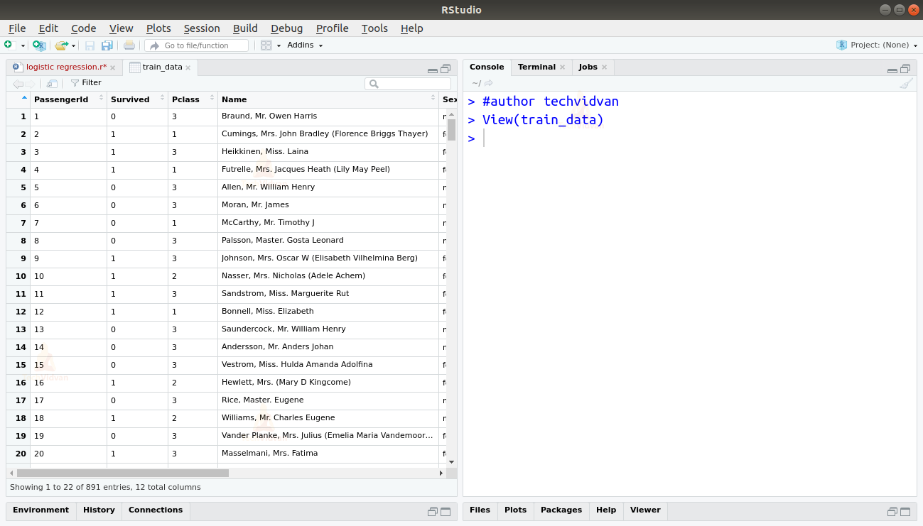
2. Let us take a look at the datasets and try to understand them.

View(train)

Output

3. The dataset consists of 12 different variables, five of which are integers, two are numeric and five are character variables.

str(train_data)

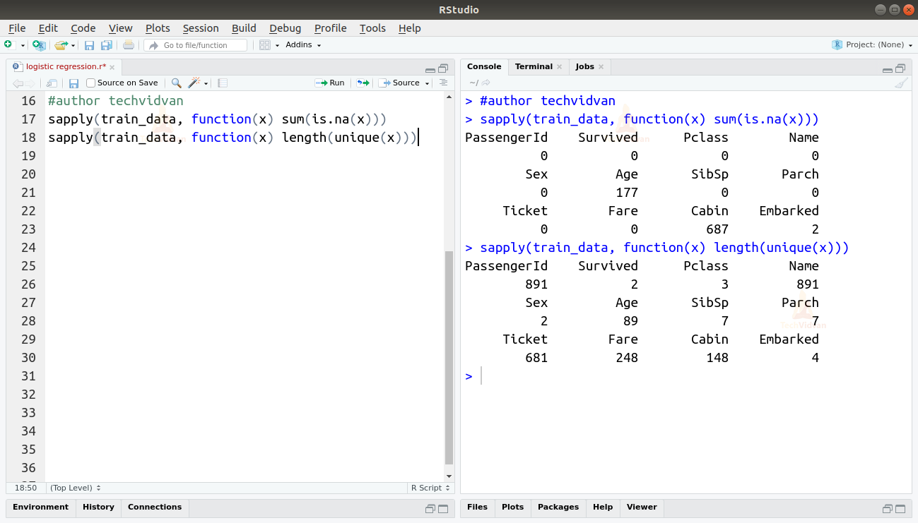
4. The dataset also contains empty values.

sapply(train_data, function(x) sum(is.na(x)))
sapply(train_data, function(x) length(unique(x)))

Output

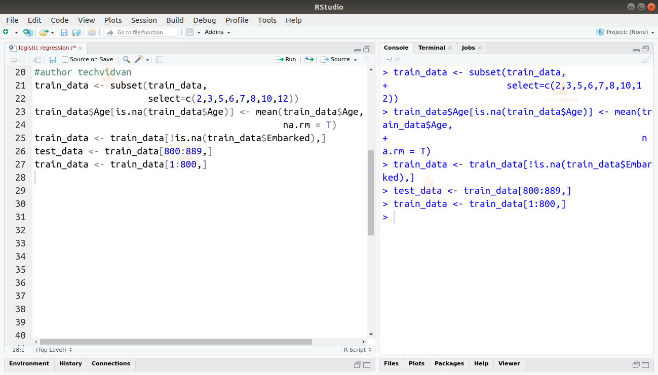
5. The variable cabin has too many empty entries. Also the variables PassengerId, Name, and Ticket only provide indexing and no further information. So we will drop these three variables. Age also has a lot of missing entries. We can replace these missing entries with an average of the rest of the entries. As Embarked has only two missing entries, it would be very easy to just omit the to incomplete rows. Finally, let’s split this cleaned data into two parts for training our model and then testing it.

train_data <- subset(train_data,
                     select=c(2,3,5,6,7,8,10,12))
train_data$Age[is.na(train_data$Age)] <- mean(train_data$Age, na.rm = T)
train_data <- train_data[!is.na(train_data$Embarked),]
test_data <- train_data[800:889,]
train_data <- train_data[1:800,]

Output

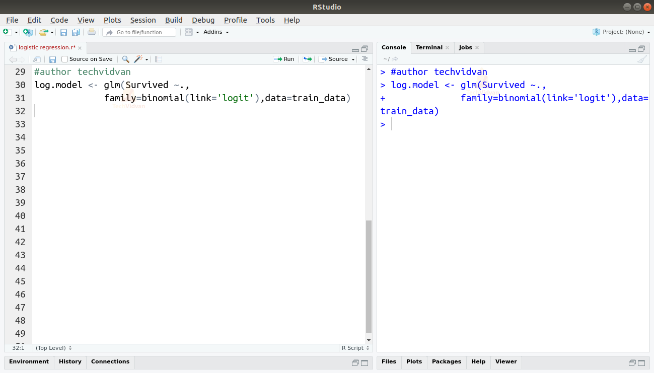
6. Now let’s fit our model. We will be using the glm() function for this. We can use the glm function to fit a logistic model by setting family = binomial.

log.model <- glm(Survived ~.,
             family=binomial(link='logit'),data=train_data)

Output

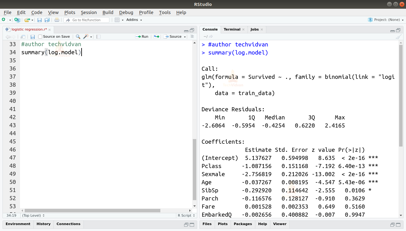
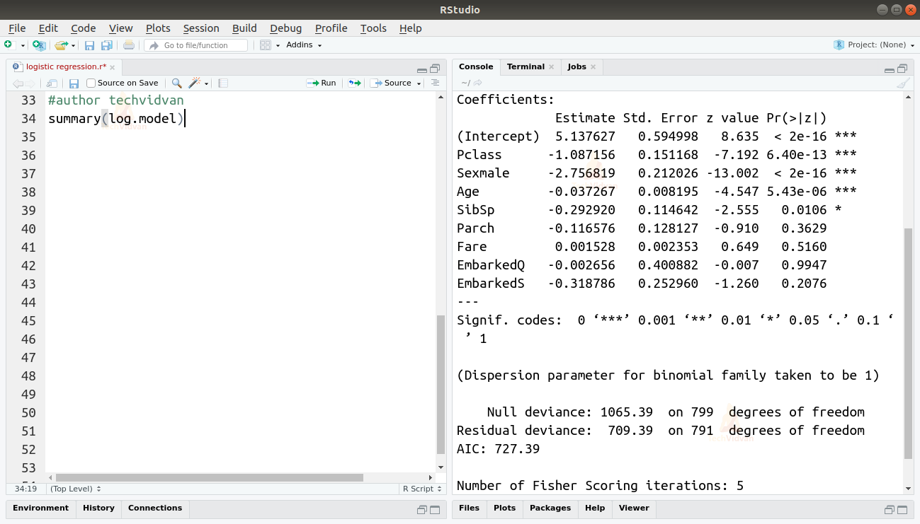
7. Finally Let us take a look at the model.

summary(log.model)

Summary

Finally, In this chapter of TechVidvan’s R tutorial series, we learned about R logistic regression models. We studied how logistic models are fit. Further we also looked at their various types. Finally, we saw a practical implementation where we fit a logistic model to a dataset.

Do share your feedback in the comment section.