R Statistics – Learning Statistics with R for Data Science
The entire data science and data analysis process involve statistics to different extents. Today, we are going to explore the basics of statistics used in data science. These are some essential concepts that data scientists use every day.
“It’s easy to lie with statistics. It’s hard to tell the truth without statistics.” – By Andrejs Dunkels
Basic Statistics in R
Being a data scientist is not just about knowing how to use data analysis tools. It also requires a good knowledge of statistics in R as well. The knowledge of elementary concepts like types of data and categories of statistical analysis is key to formulating proper plans for collecting and formatting data. Other concepts like similarity, dissimilarity, and correlation are essential for any data analysis strategy.
Wait! Have you checked packages in R?
Quantitative vs Qualitative Data
There are many ways to categorize statistical data in R. The most common one is to classify it based on whether the data is numeric or not. We can divide the data into two categories based on this:
- Quantitative data
- Qualitative data
1. Quantitative Data
Quantitative data (also known as numeric data) is data with numeric values. This type of data gives us the idea of certain quantities. We can perform arithmetic operations on quantitative data. Examples of quantitative data would be a person’s height, weight, income, blood pressure, IQ, etc..
We can further categorize quantitative data as discrete or continuous.
- Discrete: Discrete data represents items that can be counted with whole numbers (integers). In an interval, there are a limited number of values discrete data can take. The number of people in a class, the number of products in the inventory, members of a family are all examples of discrete numeric data.
- Continuous: Continuous data represent quantities that can take decimal values. These values can continue on and on in an interval. For example, a person’s weight can be 80kg, it can also be 80.5kg, 80.45kg, or 80.565kg. Here is another example, the amount of water in a 500ltr tank can be anywhere between 0 and 500. It can be 455.55ltr, 346.219ltr, or any such value. We cannot count the number of values such quantities can take.
Note: A simple way to describe the difference between discrete and continuous data would be that we can count discrete data, but we can only measure continuous data.
2. Qualitative Data
Qualitative data is data without mathematical meaning. This type of data represents the qualities or characteristics of objects. For example, the gender of a person, the color of their eyes, the flavor of a cake, etc.
Qualitative data is also called categorical data. This is because, in most cases, there is a distinct number of possible values that the variables can take.
Types of Measurement Scales
Scales of measurement are ways in which we classify variables. These classifications help with selecting appropriate collection and analysis techniques for the data. There are four types of measurement scales:
- Nominal scale
- Ordinal scale
- Interval scale
- Ratio scale
1. Nominal scale variables
Nominal scale variables are also known as categorical variables. They are the first level of measurement scales. They have distinct values to them, but these values don’t have any quantitative meaning. In R, this scale is generally used for classifications.
An example of this scale would be ‘what brand of phone do you use?’. The answer would be one of the brands that manufacture smartphones like ‘Apple,’ ‘Samsung,’ ‘Asus,’ ‘OnePlus,’ etc. These values have distinct meanings, but quantitatively one is no different than the other. We can assign them numeric values like ‘1’, ‘2’, ‘3’, or ‘4’ for easier classification, but arithmetic operations on these values are meaningless.
2. Ordinal scale variables
The ordinal scale is the second level of the measurement scales. These variables are one step further than nominal variables. They have a definite order to them. The difference between any two values is still not meaningful, but one is definitely more preferred than the other.
An example of the ordinal scale variables would be ratings. Imagine a customer service survey asking, ‘how likely are you to recommend our services to others?’. The possible answers are:
- Very unlikely
- Unlikely
- Neutral
- Likely
- Very likely
The values 1-5 assigned to these options are arbitrary. But the higher the value, the positive is the answer (in this case). The difference between any two values tells us how apart or how dissimilar the two answers are but not much else. Yet, ordinal variables give us more information than nominal variables.
3. Interval scale variables
The interval scale variables are one more step further than ordinal variables. They are the third level of the measurement scales. Interval variables have numeric values. They have a definite order to them, and also the difference or interval between any two consecutive values is constant.
A good example of interval scale variables would be Celsius or Fahrenheit temperatures. The difference between 30oC and 40oC is the same as the difference between 40oC and 50oC.
We can use techniques like mean, mode, median, and other statistical and mathematical operations to get more information from interval scale variables. They enable many techniques for proper and easier statistical analysis.
The only downside to the interval scale is that it does not have an absolute zero value. For example, while the temperature scale in oC or oF may have ‘0’ but it does not mean the absence of temperature or absence of heat. Negative values exist, and that means 0 is still a distinct value.
Interval variables are very important for correlation regression analysis and descriptive statistics in R.
4. Ratio scale variables
The ratio scale is the fourth level of measurement scale. These variables have all the properties of the interval variables, and they also have a pre-defined starting value which signifies true zero.
A person’s height or weight are good examples of ratio scale variables. They have all the properties of the interval variables such as their values are ordered and the difference between the values is constant. Apart from that, they also have a true zero. A person’s height or weight cannot be negative. A ‘0’ on the weight scale signifies an absence of weight.
We can use measures like mean, median, and mode to find the central tendencies of ratio variables. Quantitative analysis techniques like SWOT, cross-tabulation, geometric mean, harmonic mean, etc. are also useful on them.

Types of Statistical Analysis
Statistics in R can be categorized into two main branches. These are:
- Descriptive statistics
- Inferential statistics
1. Descriptive statistics
Descriptive statistics deals with describing the data. It describes the properties of data using measures like mean, median, dispersion, variance, central tendency, skewness, etc. Descriptive statistics deals with improving our understanding of the data by describing or summarizing it.
Imagine we have the details of students in a school. We know their names, ages, gender, their annual family incomes, their average scores, etc. We can find the mean of their family incomes, which would give us an understanding of the average financial condition of a student in that particular school. The ratio of male count vs. the female count can tell us about the gender ratio in the school. Descriptive statistics deals with summarizing the existing data to give a better understanding.
2. Inferential statistics
Inferential statistics deals with using existing data to make predictions regarding a larger population. It uses techniques like hypothesis testing, regression analysis, analysis of variance, and confidence intervals on sample data to make probabilistic predictions about a larger population.
Suppose, we need to find the average scores of school-going children in the entire city. Gathering data for the entire city would be a difficult task. Instead, we can use the data from the single school as a sample and try to predict the required ratio. Inferential statistics cannot provide accurate answers, but it can give us ranges and estimates where the actual answers and values may fall.
Proximity Measures
We use proximity measures in data mining and machine learning to measure how alike or how unalike two objects are. Data mining techniques like clustering, anomaly detection, and nearest neighbor locating use them. The term proximity can mean similarity or dissimilarity measures.
1. Similarity
The similarity is a measure of likeness between two objects. It measures how alike any two objects are. The similarity measure can have a value from 0 (no similarity) to 1 (completely similar). The similarity between two objects p and q is referred to as s(p,q).
2. Dissimilarity
Dissimilarity is the measure of how unlike or different the two objects are. It is also called distance. The dissimilarity measure can take values from 0 (objects are similar) to ∞ (objects are completely different). The dissimilarity between two objects p and q is referred to as d(p,q).
As dissimilarity is synonymous with distance, we can use various distance measures to calculate the distance or dissimilarity between two objects. The most commonly used distance measures are:
Euclidean distance: The Euclidean distance between two points is the shortest distance between them. The formula for it is derived from the Pythagoras theorem.
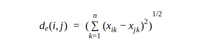
Where i and j are the ith and jth objects and xik and xjk are the kth attributes of i and j.

Minkowski distance: The Minkowski distance formula generalizes the Euclidean distance.
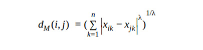
Where λ is the number of dimensions.
Mahalanobis distance: Let α be an N x p matrix. Then the ith row of α would be

Then the Mahanalobis distance between i and j would be
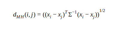
Where Σ is p x p sample covariance matrix.
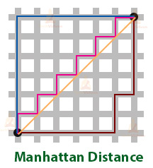
Manhattan distance: Manhattan distance is also known as city-block distance. We calculate it by traversing from the first point to the second in a horizontal and vertical grid.

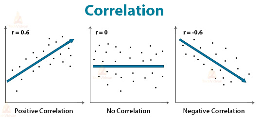
Correlation
Correlation measures the relationship between two variables. It shows whether and how strong is the connection between two variables. Correlation measure takes a value between -1 and 1.
If the value is closer to +1, then the relation is positive. This means that an increase in one variable increases the other variable as well.
If the value is closer to -1, the relation is negative. This means that an increase in one variable decreases the other variable.
If the value is close to 0, this means that there is no relation between the two variables.
Summary
A data scientist is a mixture of a computer programmer and a statistician. Statistics in R play a vital and ever-present role in data science and analytics. In the R tutorial, we studied a few basic concepts of statistics that are commonly used for data science and data analysis with R.
Any difficulty while practicing statistics in R programming?
Ask our TechVidvan experts.
Keep practicing buddy!!