Diabetes Prediction using Machine Learning
With this Machine Learning Project, we will be doing diabetes prediction analysis. For this project, we are using the Random Forest Classifier, Support Vector Classifier, and Gradient Boosting Algorithm.
So, let’s build this system.
Diabetes Prediction
Diabetes is one of the toughest illnesses. Diabetes is developed as a result of various conditions, including obesity and high blood sugar. It has an effect on the insulin hormone, which makes crabs’ metabolisms erratic and elevates blood sugar levels. Diabetes is developed when the body does not create enough insulin.
The World Health Organization estimates that 422 million people globally, mostly in low- and middle-income countries, have diabetes (WHO). And this number could rise to 490 million by the year 2030. However, diabetes rates are high in places like Canada, China, India, etc. There are 40 million diabetics in India, which has a population of over 1000 million presently. Diabetes is one of the main causes of death around the globe. Diabetes can be managed and controlled at early stages.
By utilizing a number of diabetes disease-related characteristics, we will make the prediction of diabetes. In this research, the Pima Indian Diabetes Dataset is utilized to anticipate diabetes using a variety of machine learning classification and ensemble techniques. Different machine learning algorithms provide efficient results for knowledge collecting by building numerous classifications and ensemble models from the given datasets. These findings may help in the diagnosis of diabetes. There are many different machine learning techniques that may be used to make predictions, but picking the most efficient one can be difficult. So, to make predictions, we need a dataset and run well-known classification and ensemble algorithms on it.
Choosing Model
The Random Forest algorithm, a machine learning technique, was suggested by K.Vijiya Kumar. It was designed to create a system that can predict diabetes earlier in the course of a patient’s life with more accuracy. The results indicated that the prediction system is able to forecast diabetes disease effectively, efficiently, and quickly. The suggested model yields the best results for diabetic prediction.
Diabetes Prediction was suggested by Nonso Nnamoko using an ensemble supervised learning approach in which five commonly used classifiers were utilized for the ensembles, and their outputs were combined using a meta-classifier. The results are presented and compared to those from previous studies that used the same dataset.
Studies have shown that diabetes can be cured at early stages. Tejas N. Joshi et al. produced a diabetes prediction. Using Machine Learning Approaches, he attempts to predict diabetes by employing three different supervised machine learning techniques, including SVM, Logistic Regression, and ANN. The results of his experiment point to a practical technique for early diabetic illness detection. Dheeraj Shetty suggested using data mining to anticipate diabetes disease in order to develop an Intelligent Diabetic Illness Prediction System which can analyze the condition using the data of diabetic patients. In his research, it is suggested that diabetes patient databases can be analyzed using algorithms like Bayesian and KNN (K-Nearest Neighbor), which are used to forecast the development of diabetes disease.
There are a lot of algorithms that can be used. But the Random Forest Classifier seems to perform the best for our project with an accuracy of around 90%.
Let’s have a look at the model.
Random Forest Classifier
In addition to being used for classification and regression tasks, it is also a type of ensemble learning technique. It provides a higher level of accuracy than other models. Large datasets can be handled by this strategy very easily. Leo Bremen created Random Forest. It is a well-liked collective learning approach. By lowering variance, Random Forest enhances the performance of the Decision Tree. During training, it builds a large number of decision trees, and then it outputs the class that represents the mean of all the classes.
Algorithm
- Selecting the “R” features from the total features “m” where R>M is the first step.
- The node employs the most effective split point out of all the “R” features.
- Choose the optimal split to divide the node into sub-nodes.
- Until you reach “l” number of nodes, repeat steps a through c.
- By performing steps a through d repeatedly, you can build a forest by adding “a” number of trees to “n” trees.
Project Prerequisites
The requirement for this project is Python 3.6 installed on your computer. I have used a Jupyter notebook for this project. You can use whatever you want.
The required modules for this project are –
- Numpy(1.22.4) – pip install numpy
- Pandas(1.5.0) – pip install pandas
- Seaborn(0.9.0) – pip install seaborn
- SkLearn(1.1.1) – pip install sklearn
Diabetes Prediction Project & DataSet
We have provided the diabetes prediction project source code as well as dataset for this project that will be required in this ml project. We will require a csv file for this project. You can download the dataset and the jupyter notebook from the link below.
Download the dataset and the jupyter notebook from the following link: Diabetes Prediction Project
Steps to Implement
1. Import the modules and the libraries. For this project, we are importing the libraries numpy, pandas, seaborn, sklearn and matplotlib.
import numpy as np #importing the numpy library which will be used in this project
import pandas as pd #importing the pandas library which will be used in this project
import matplotlib.pyplot as plt
import seaborn as sns#importing the seaborn library which will be used for plotting the heatmaps
from sklearn.model_selection import train_test_split#importing the test_train_split library from sklearn model_selection which will be used in this project
from sklearn.metrics import confusion_matrix, accuracy_score#importing the confusion matrix from sklearn.metrics library which will be used in this project
from sklearn.svm import SVC#importing the SVC from sklearn.svm library which will be used in this project
from sklearn.ensemble import RandomForestClassifier#importing the Random Forest Classifier library which will be used in this project
from sklearn.ensemble import GradientBoostingClassifier#importing the Gradient Boosting Classifier library which will be used in this project
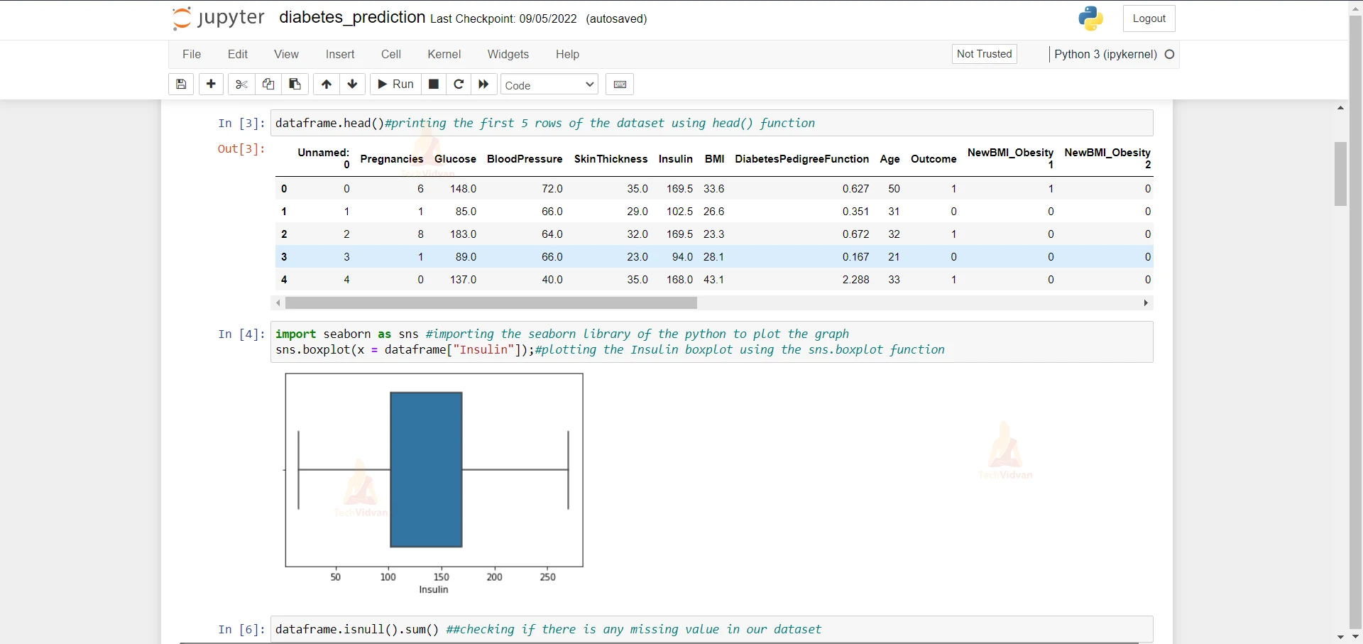
2. Here we are reading our dataset. And we are printing our dataset
dataframe = pd.read_csv('dataset.csv') ##reading the csv file of the diabetes dataset

dataframe.head()#printing the first 5 rows of the dataset using head() function
3. Here we are importing the seaborn library and we are plotting a box plot of insulin column.
import seaborn as sns #importing the seaborn library of the python to plot the graph
sns.boxplot(x = dataframe["Insulin"]);#plotting the Insulin boxplot using the sns.boxplot function
4. Here we are checking if there is any null value in the data. As we can see that there are no null values in the dataset.
dataframe.isnull().sum() ##checking if there is any missing value in our dataset
5. Here we are printing the dataset again.
dataframe.head() #as there is no missing value in our dataset and we are printing our datset again
6. Here we are printing the correlation of the dataset to see which column is the most irrelevant.
dataframe.corr() #printing the correlation of the dataframe to see the correlation of every column
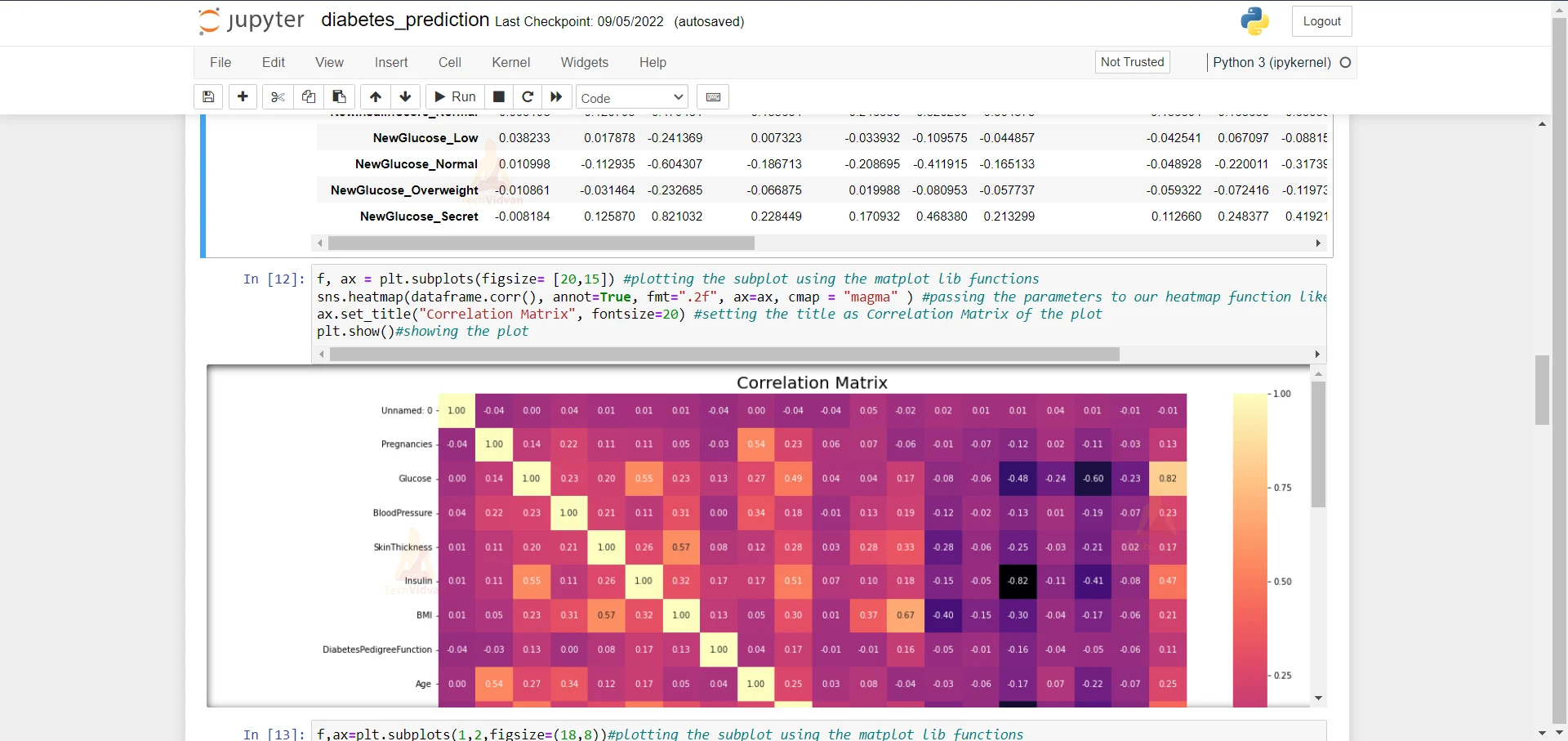
7. Here we are plotting the heatmap to see the correlation more clearly using seaborn library. We are using the heatmap function of the seaborn library.
f, ax = plt.subplots(figsize= [20,15]) #plotting the subplot using the matplot lib functions
sns.heatmap(dataframe.corr(), annot=True, fmt=".2f", ax=ax, cmap = "magma" ) #passing the parameters to our heatmap function like cmap = magma and annot = True
ax.set_title("Correlation Matrix", fontsize=20) #setting the title as Correlation Matrix of the plot
plt.show()#showing the plot
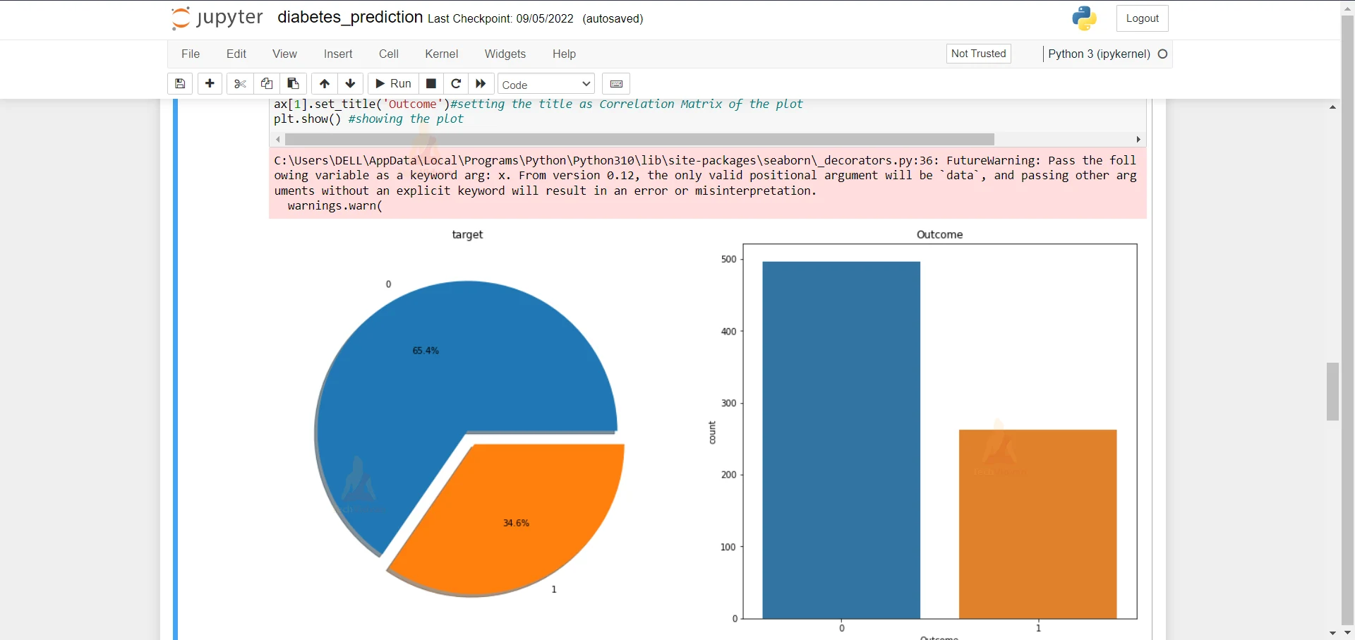
8. Here we are plotting a pie chart and a countplot of the ‘Target’ column and the ‘Outcome’ column.
f,ax=plt.subplots(1,2,figsize=(18,8))#plotting the subplot using the matplot lib functions
dataframe['Outcome'].value_counts().plot.pie(explode=[0,0.1],autopct='%1.1f%%',ax=ax[0],shadow=True)#plotting the subplot using the matplot lib functions
ax[0].set_title('target')#setting the title as Correlation Matrix of the plot
ax[0].set_ylabel('')#setting the title as Correlation Matrix of the plot
sns.countplot('Outcome',data=dataframe,ax=ax[1])
ax[1].set_title('Outcome')#setting the title as Correlation Matrix of the plot
plt.show() #showing the plot
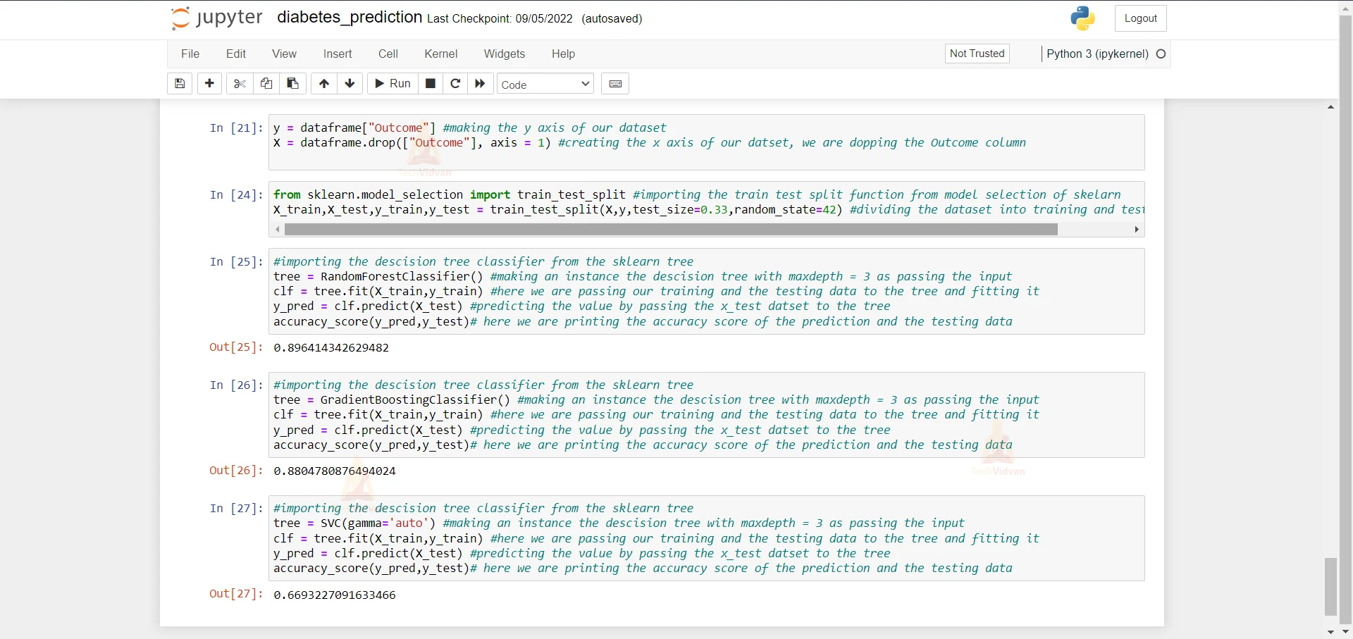
9. Here we are creating the x and the y dataset from our original dataset.
y = dataframe["Outcome"] #making the y axis of our dataset
X = dataframe.drop(["Outcome"], axis = 1) #creating the x axis of our datset, we are dopping the Outcome column
10. Here we are importing the train test split function from sklearn and then we are dividing the dataset into training and testing.
from sklearn.model_selection import train_test_split #importing the train test split function from model selection of skelarn
X_train,X_test,y_train,y_test = train_test_split(X,y,test_size=0.33,random_state=42) #dividing the dataset into training and testing dataset
11. Here we are importing the Random forest Classifier and we are passing our training and testing dataset to see it and see what is the accuracy of this algorithm. The accuracy of this algorithm comes out to be 89%.
#importing the descision tree classifier from the sklearn tree
tree = RandomForestClassifier() #making an instance the descision tree with maxdepth = 3 as passing the input
clf = tree.fit(X_train,y_train) #here we are passing our training and the testing data to the tree and fitting it
y_pred = clf.predict(X_test) #predicting the value by passing the x_test datset to the tree
accuracy_score(y_pred,y_test)# here we are printing the accuracy score of the prediction and the testing data
12. Here we are importing the Gradient Boosting Classifier and we are passing our training and testing dataset to see it and see what is the accuracy of this algorithm. The accuracy of this algorithm comes out to be 88%.
#importing the decision tree classifier from the sklearn tree
tree = GradientBoostingClassifier() #making an instance the descision tree with maxdepth = 3 as passing the input
clf = tree.fit(X_train,y_train) #here we are passing our training and the testing data to the tree and fitting it
y_pred = clf.predict(X_test) #predicting the value by passing the x_test datset to the tree
accuracy_score(y_pred,y_test)# here we are printing the accuracy score of the prediction and the testing data
13. Here we are importing the Support Vector Classifier and we are passing our training and testing datasets to see it and see what is the accuracy of this algorithm. The accuracy of this algorithm comes out to be 66%.
#importing the descision tree classifier from the sklearn tree
tree = SVC(gamma='auto') #making an instance the descision tree with maxdepth = 3 as passing the input
clf = tree.fit(X_train,y_train) #here we are passing our training and the testing data to the tree and fitting it
y_pred = clf.predict(X_test) #predicting the value by passing the x_test datset to the tree
accuracy_score(y_pred,y_test)# here we are printing the accuracy score of the prediction and the testing data
Summary
In this Machine Learning project, we develop diabetes prediction. For this project, we are using the Random Forest Classifier, Support Vector Classifier, and Gradient Boosting Algorithm. We hope you have learned something new in this project.