Machine Learning Parkinson’s Disease Detection Project

What is Parkinson’s Disease?

Parkinson’s disease is a progressive disorder that affects the nervous system and the parts of the body controlled by the nerves. Symptoms start slowly. The first symptom may be a barely noticeable tremor in just one hand. Tremors are common, but the disorder may also cause stiffness or slowing of movement.

In the early stages of Parkinson’s disease, your face may show little or no expression. Your arms may not swing when you walk. Your speech may become soft or slurred. Parkinson’s disease symptoms worsen as your condition progresses over time.

Although Parkinson’s disease can’t be cured, medications might significantly improve your symptoms. Occasionally, your healthcare provider may suggest surgery to regulate certain regions of your brain and improve your symptoms.

Dataset

The Parkinson’s Disease Data Set is a comprehensive collection of data that provides clinical, demographic, and behavioural information from Parkinson’s disease patients. This data is obtained from diverse sources, including neuroimaging data, clinical assessments, wearable sensors etc.

With a total of 195 observations and 24 features, this dataset includes variables such as Average vocal fundamental frequency, the health status of the subject, signal fractal scaling exponent etc. Exploratory Data Analysis is carried out on the dataset to identify any potential outliers, as well as to get some detailed information about the data. In the next step, the data can be used to train Machine Learning models, then make predictions depending on the input. The Parkinson’s Disease Data Set is available for download on Kaggle.

Tools and Libraries Used

The project makes use of the following Python libraries:

• NumPy
• Pandas
• Matplotlib
• Seaborn
• Scikit-Learn

Download Machine Learning Parkinson’s Disease Detection Project

Please download the source code of Machine Learning Parkinson’s Disease Detection Project from the following link: Machine Learning Parkinson’s Disease Detection Project Code.

Steps for Detecting Parkinson’s Disease Using Machine Learning

You must complete a set of steps in order to create this Machine Learning Parkinson’s Disease Detector. We are here to walk you through every stage of developing an app.

1. Importing the required libraries.

import numpy as np
import pandas as pd
import matplotlib.pyplot as plt
import seaborn as sns
sns.set_style('darkgrid')

2. Once the necessary libraries have been imported, the next step would be to read the dataset and display the dataset as well. The first five rows have been displayed in the screenshot shown below.

parkinson_data = pd.read_csv("parkinsons.data")
parkinson_data.head()`

Output:

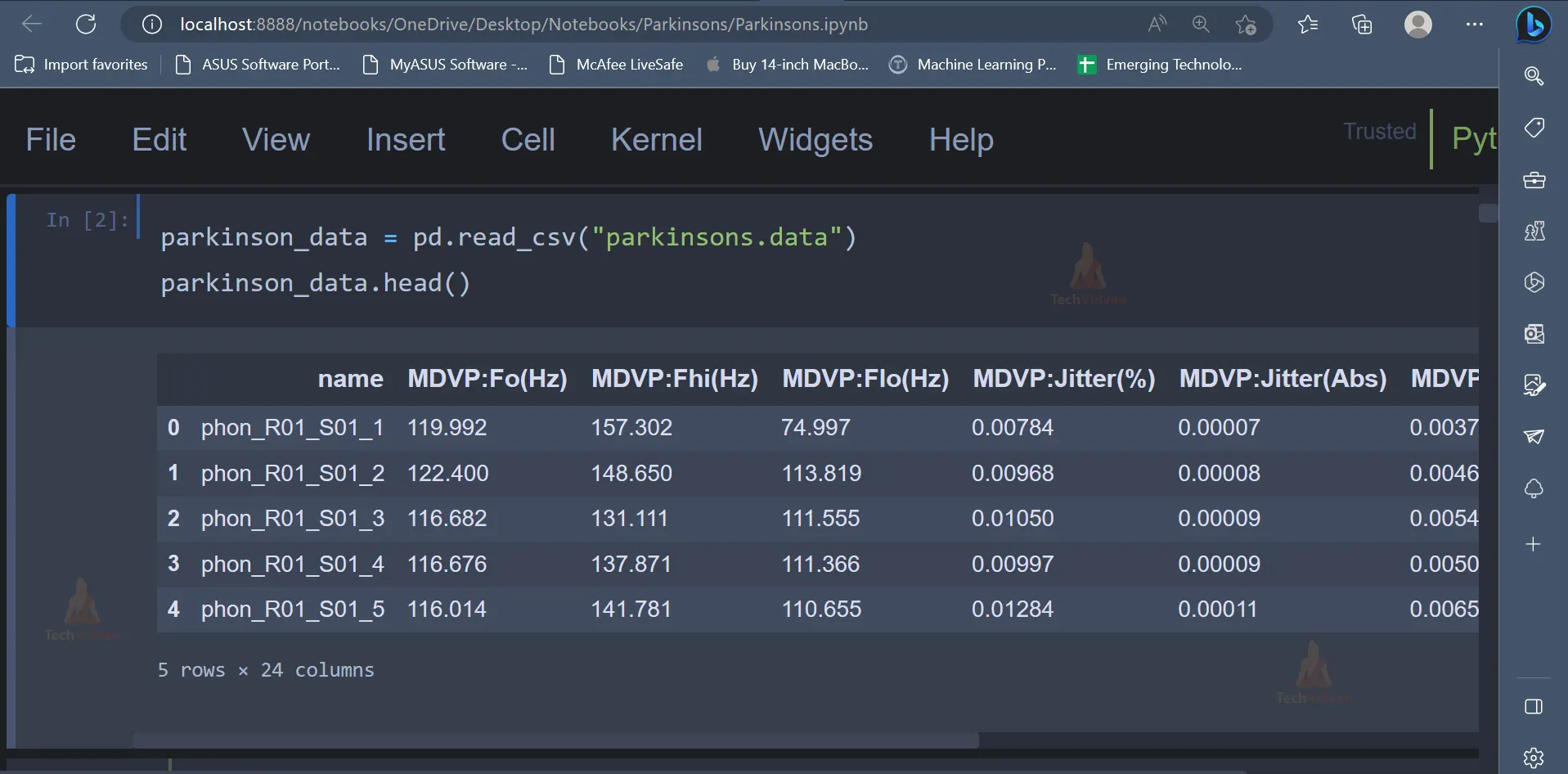
3. The dataset contains multiple columns, which can be seen above. Let’s understand what is the meaning of each attribute/column present in the dataset.

Attributes:

• name – ASCII subject name and recording number
• MDVP:Fo(Hz) – Average vocal fundamental frequency
• MDVP:Fhi(Hz) – Maximum vocal fundamental frequency
• MDVP:Flo(Hz) – Minimum vocal fundamental frequency
• MDVP:Jitter(%), MDVP:Jitter(Abs), MDVP:RAP, MDVP:PPQ, Jitter:DDP – Several measures of variation in fundamental frequency
• MDVP:Shimmer,MDVP:Shimmer(dB),Shimmer:APQ3,Shimmer:APQ5,MDVP:APQ,Shimmer:DDA – Several measures of variation in amplitude
• NHR, HNR – Two measures of the ratio of noise to tonal components in the voice
• status – The health status of the subject (one) – Parkinson’s, (zero) – healthy
• RPDE, D2 – Two nonlinear dynamical complexity measures
• DFA – Signal fractal scaling exponent
• spread1,spread2,PPE – Three nonlinear measures of fundamental frequency variation

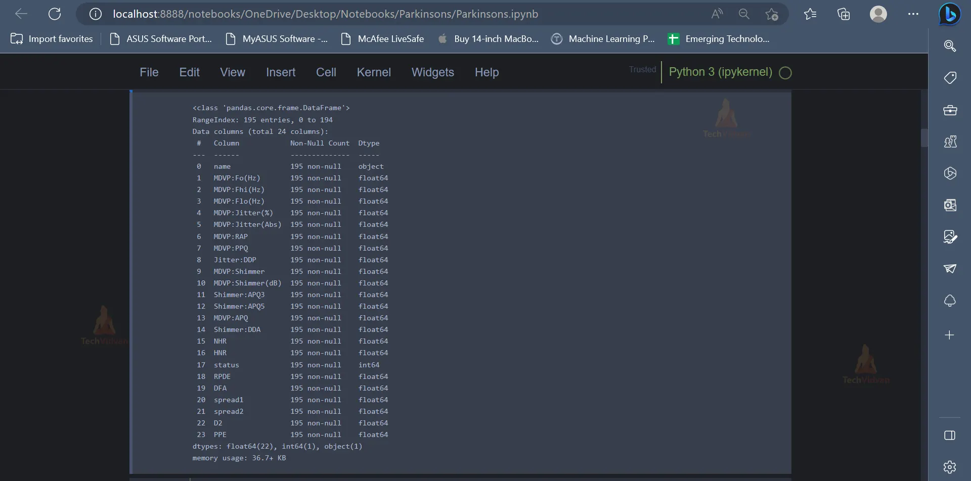
4. Now that there is a clear understanding of the various attributes present in the dataset, the next step would be to use exploratory data analysis to gain more insights as well as discover some hidden patterns or trends present in the dataset.

parkinson_data.info()

Output:

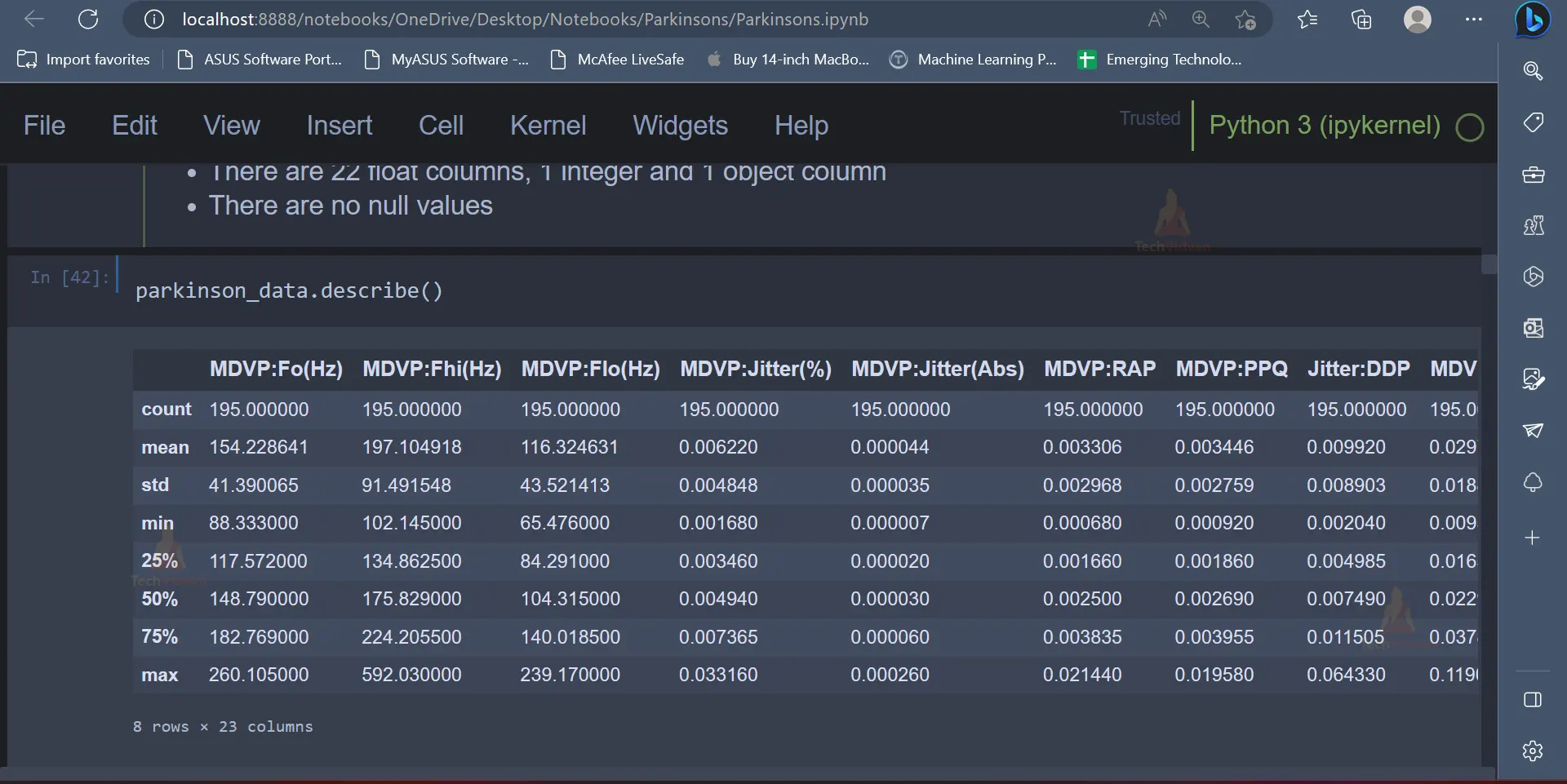
5. Datasets usually contain extreme values, which are usually called outliers. Outliers present in the dataset can be analysed using the below code. There are some outliers. As we can see, some attributes have huge differences in their 75-percentile value and maximum value, which is evident from the below output.

parkinson_data.describe()

Output:

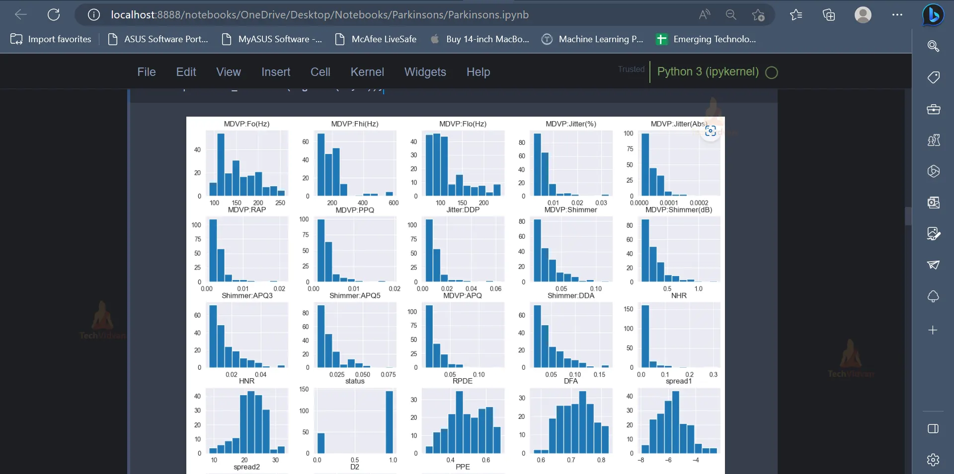
6. After exploring the dataset and the various features, one can use data visualisation concepts to present the data and the trends present in the data in a visually appealing format. Data Visualization techniques like pie charts, dist-plot etc. can be used for this purpose.

parkinson_data['status'].value_counts().plot(kind='pie', autopct = "%1.0f%%")
plt.title("Distribution in the 'status' Column")
plt.show()

Output:

parkinson_data.hist(figsize=(15,12));``

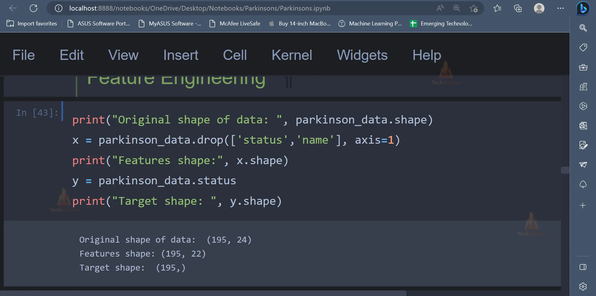
7. After representing the data visually, it is now time to perform Feature Engineering, to select the required features which will be used to train the Machine Learning model.

print("Original shape of data: ", parkinson_data.shape)
x = parkinson_data.drop(['status','name'], axis=1)
print("Features shape:", x.shape)
y = parkinson_data.status
print("Target shape: ", y.shape)

Output:

8. The dataset contains attributes which belong to a wide range. It would be convenient to have all the values belonging to a similar range or a similar scale which would eventually help the machine learning model understand the data in a better way. The MinMaxScaler can be used for this purpose, as shown below.

from sklearn.preprocessing import MinMaxScaler
scaler = MinMaxScaler((-1, 1))
# fits the data to the MinMaxScaler
X = scaler.fit_transform(x)

The primary purpose of utilising MinMaxScaler is to standardise feature scales and bring them to a similar level, leading to enhanced performance of specific machine learning algorithms. This technique is especially beneficial for algorithms that utilise distance calculations, like support vector machines or k-nearest neighbours.

9. In the next step, the dataset will be split into training data and testing data. The training data will be used to train the model, and the testing data will be used to evaluate the model’s performance.

from sklearn.model_selection import train_test_split
x_train, x_test, y_train, y_test=train_test_split(X, y, test_size=0.2) 

10. Now that the data is split into training data and testing data, various machine learning models can be trained using the training data. We will be using models like Logistic Regression, Decision Trees, Random Forest Classifier etc.

from sklearn.linear_model import LogisticRegression
# Importing the Logistic Regression and creating an instance of it
clf = LogisticRegression()
#Train Model
clf.fit(x_train, y_train)


# Prediction on Test and Train Set 
pred_logistic_test = clf.predict(x_test)
pred_logistic_train = clf.predict(x_train)

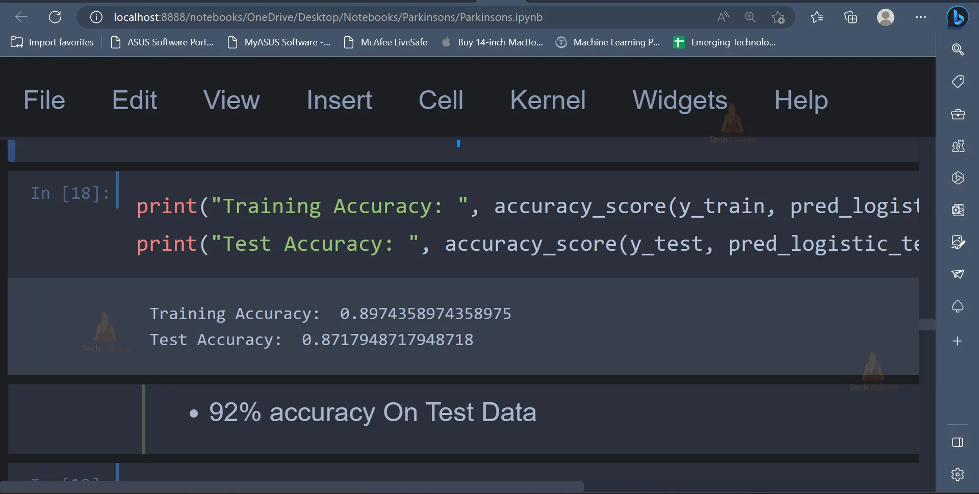
11. Once the model is trained, the model’s performance can be tested using various metrics like confusion matrix, classification report, accuracy score etc.

from sklearn.metrics import confusion_matrix,accuracy_score, classification_report
print("Training Accuracy: ", accuracy_score(y_train, pred_logistic_train))
print("Test Accuracy: ", accuracy_score(y_test, pred_logistic_test))

Output:

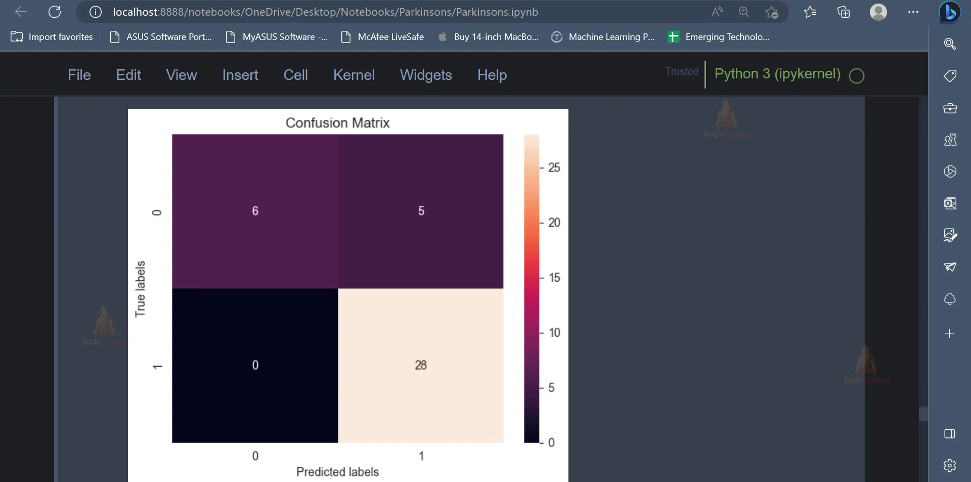
cm = confusion_matrix(y_test, pred_logistic_test)
ax= plt.subplot()
sns.heatmap(cm, annot=True, ax = ax);
ax.set_xlabel('Predicted labels')
ax.set_ylabel('True labels') 
ax.set_title('Confusion Matrix')
plt.show()

Output:

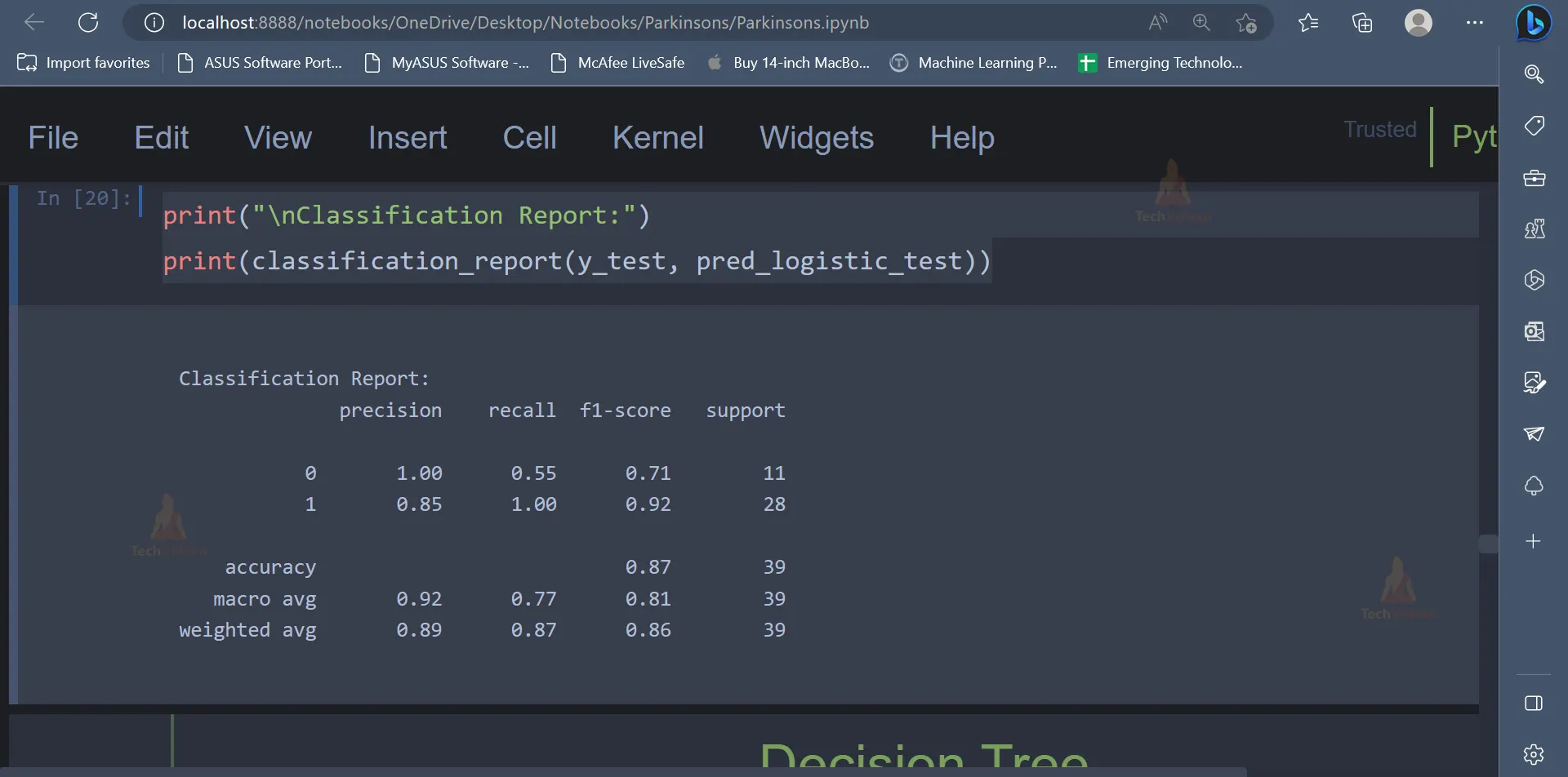
print("\nClassification Report:")
print(classification_report(y_test, pred_logistic_test))

Output:

12. The next model, which we will be using is the Decision Tree Classifier.

from sklearn.tree import DecisionTreeClassifier
dt = DecisionTreeClassifier()
# Train model 
dt.fit(x_train, y_train)


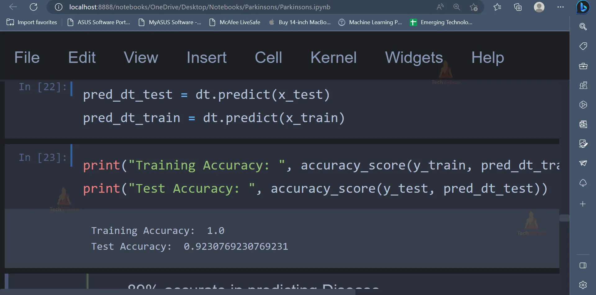
pred_dt_test = dt.predict(x_test)
pred_dt_train = dt.predict(x_train)
# Making predictions using the data


print("Training Accuracy: ", accuracy_score(y_train, pred_dt_train))
print("Test Accuracy: ", accuracy_score(y_test, pred_dt_test))

Output:

 cm = confusion_matrix(y_test, pred_dt_test)
ax= plt.subplot()
sns.heatmap(cm, annot=True, ax = ax);
ax.set_xlabel('Predicted labels')
ax.set_ylabel('True labels') 
ax.set_title('Confusion Matrix')
plt.show()

Output: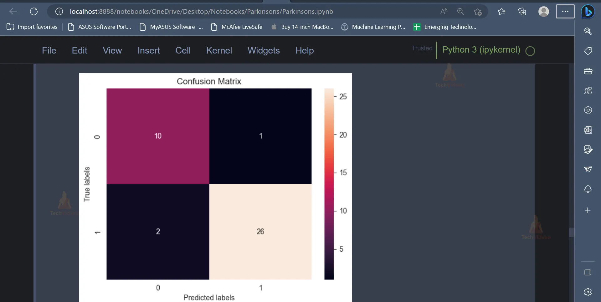

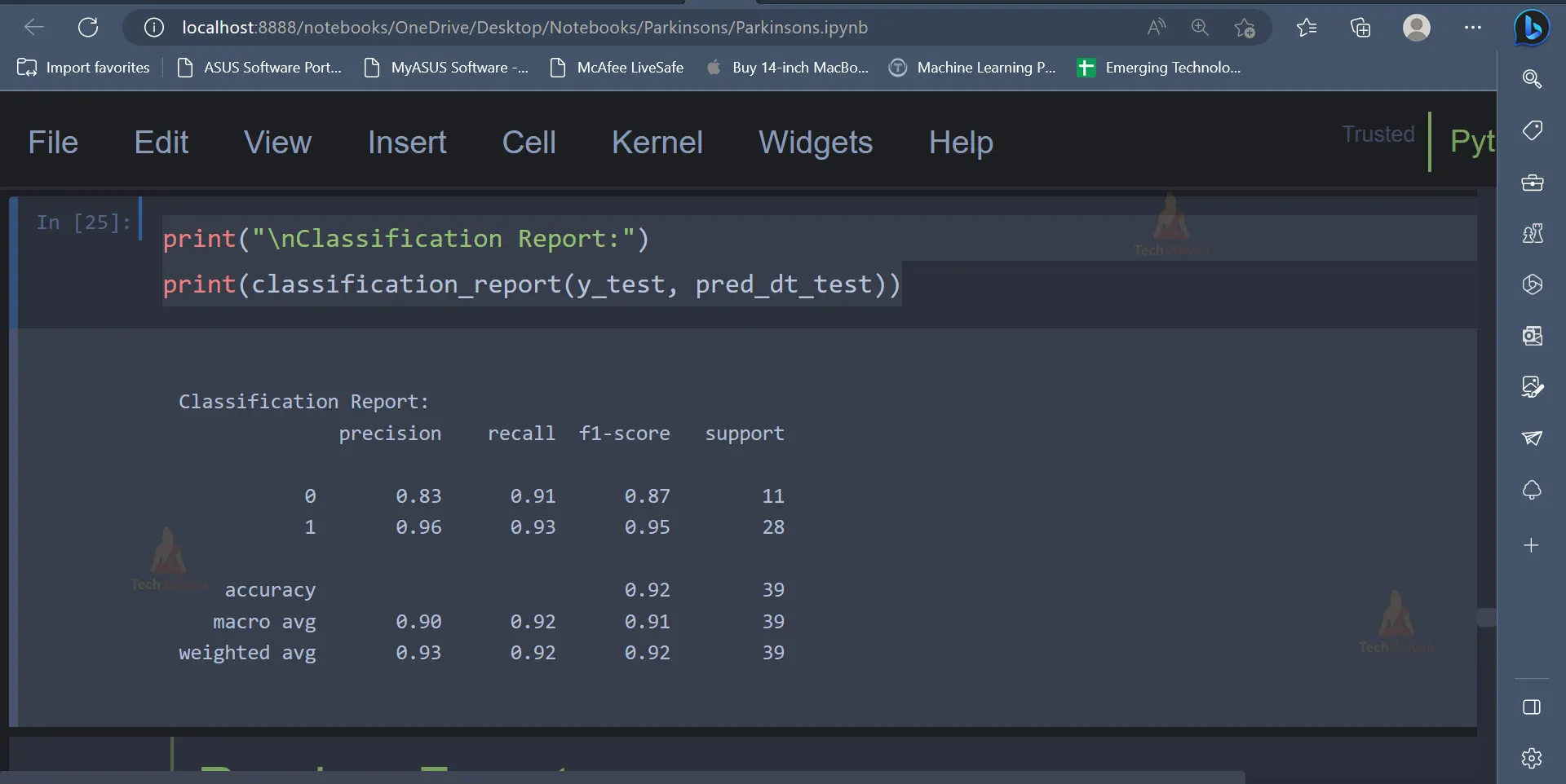
print("\nClassification Report:")
print(classification_report(y_test, pred_dt_test))

13. After the Decision Tree Classifier, the Random Forest Classifier can be used to predict whether a person will have Parkinson’s disease or not.

from sklearn.ensemble import RandomForestClassifier
rf = RandomForestClassifier()
rf.fit(x_train, y_train)


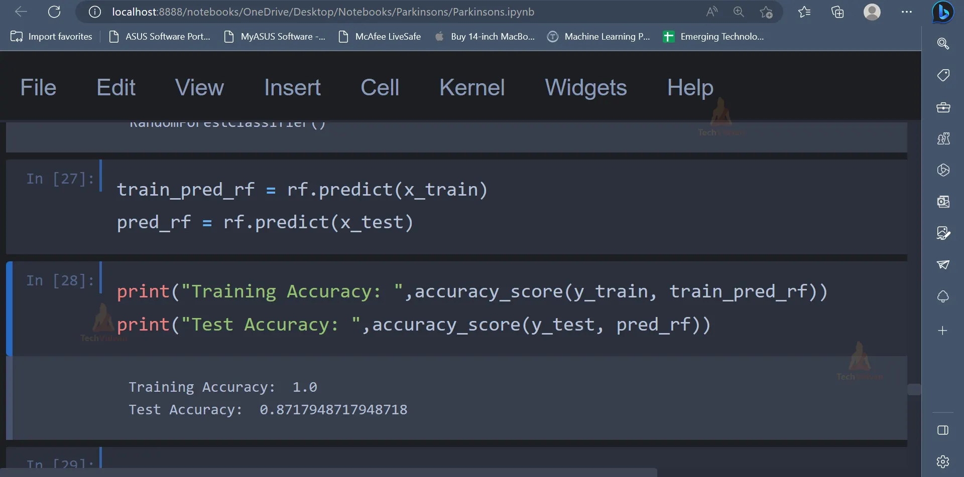
train_pred_rf = rf.predict(x_train)
pred_rf = rf.predict(x_test)


print("Training Accuracy: ",accuracy_score(y_train, train_pred_rf))
print("Test Accuracy: ",accuracy_score(y_test, pred_rf))

Output:

cm = confusion_matrix(y_test, pred_rf)
ax= plt.subplot()
sns.heatmap(cm, annot=True, ax = ax);
ax.set_xlabel('Predicted labels')
ax.set_ylabel('True labels') 
ax.set_title('Confusion Matrix')
plt.show()

Output:

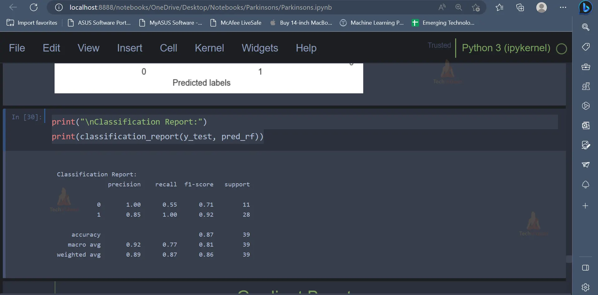
print("\nClassification Report:")
print(classification_report(y_test, pred_rf))

Output:

14. The last algorithm which will be used is the Gradient Boosting Algorithm.

from sklearn.ensemble import GradientBoostingClassifier
gb = GradientBoostingClassifier()
# Training model
gb.fit(x_train, y_train)

# Prediction on test and train set
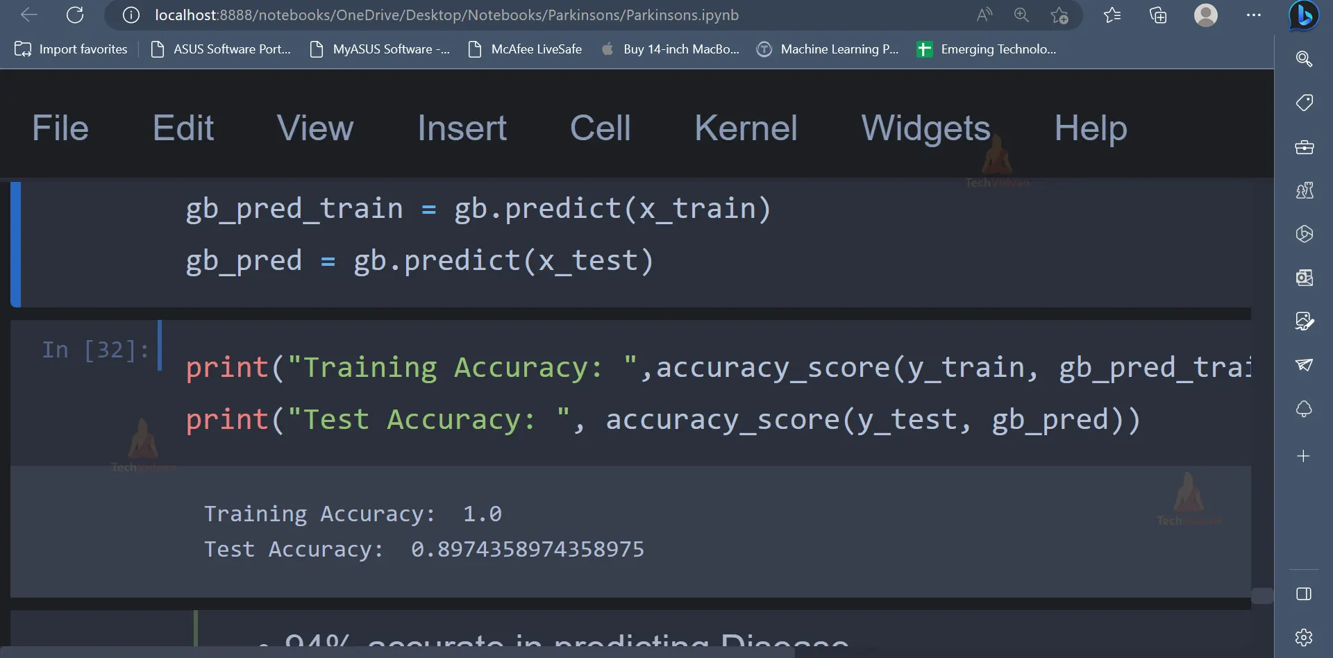
gb_pred_train = gb.predict(x_train)
gb_pred = gb.predict(x_test)


print("Training Accuracy: ",accuracy_score(y_train, gb_pred_train))
print("Test Accuracy: ", accuracy_score(y_test, gb_pred))

Output:

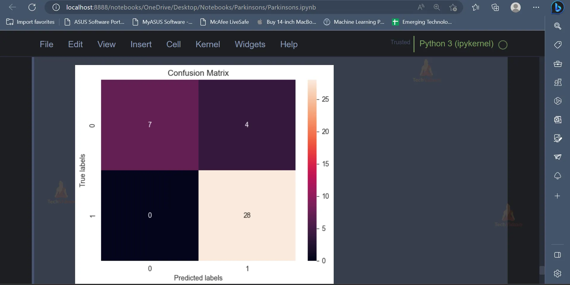
cm = confusion_matrix(y_test, gb_pred)
ax= plt.subplot()
sns.heatmap(cm, annot=True, ax = ax);
ax.set_xlabel('Predicted labels')
ax.set_ylabel('True labels') 
ax.set_title('Confusion Matrix')
plt.show()

Output:

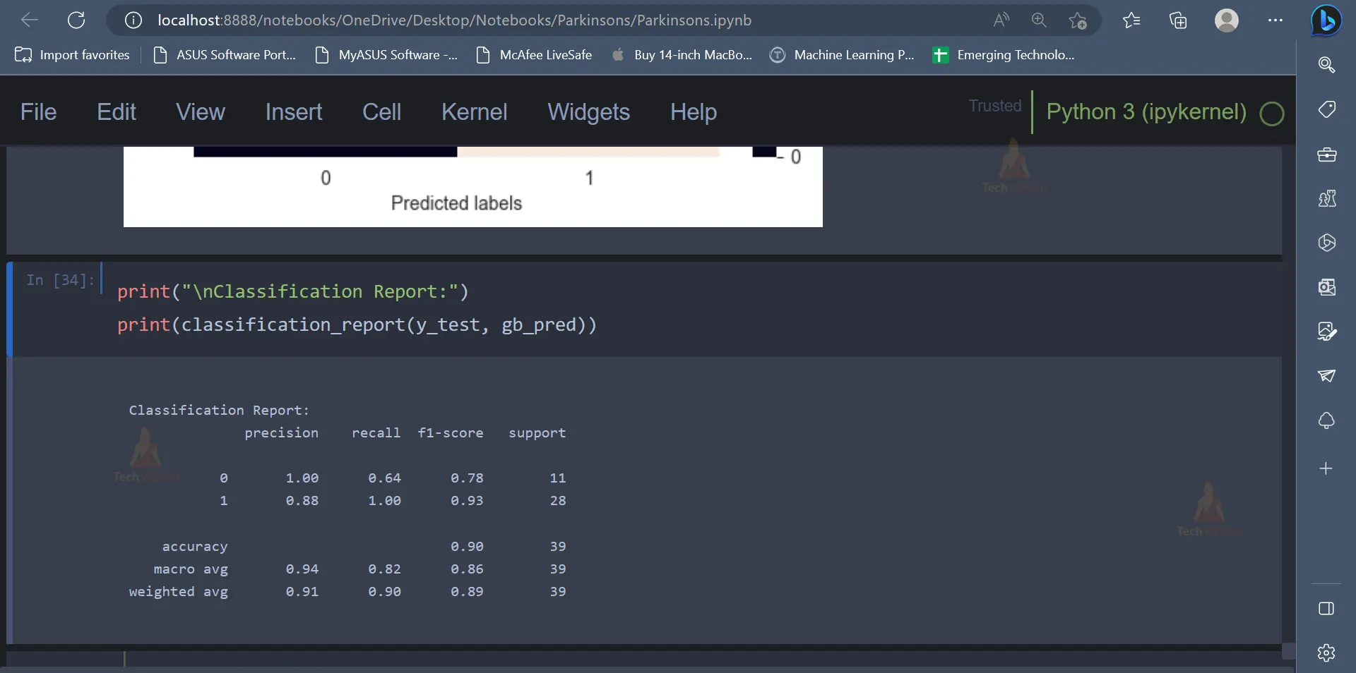
print("\nClassification Report:")
print(classification_report(y_test, gb_pred))

Output:

Conclusion

The implementation of machine learning algorithms in Parkinson’s disease detection is a promising and efficient approach. By analysing the Parkinson’s Disease Data Set, we were able to create models that can accurately predict the presence of Parkinson’s disease in a patient, with high levels of accuracy and precision.

Nevertheless, it is crucial to emphasise that these models are not a substitute for clinical assessment by trained medical professionals. Therefore, the use of machine learning algorithms for Parkinson’s disease detection should be viewed in combination with traditional diagnostic methods. Additionally, further research and development are necessary to refine the accuracy and precision of the models, as well as extend the dataset used to train them.