Machine Learning Weather Prediction – Forecasting the Future
What is a Weather Prediction?
Weather prediction, often known as weather forecasting, is the act of predicting the state of the atmosphere at a specific time and location in the future. It is a critical field of research for comprehending and forecasting the behaviour of our planet’s atmosphere, which is constantly changing owing to natural and man-made forces. Accurate weather prediction has several uses, including agriculture, transportation, aviation, and disaster management.
Because of their capacity to model complex connections and patterns in huge datasets, machine learning approaches have grown in popularity in weather prediction. With huge volumes of weather data available from multiple sources such as satellites, radars, and weather stations, machine learning systems may learn from this data to effectively anticipate weather conditions.
In this project, we will look at the many data sources utilised in weather forecasting, as well as the various machine learning methods used for weather prediction and their benefits and drawbacks. Finally, we will compare the performance of a machine learning model trained on weather data.
Dataset
The dataset used for this project contains the weather conditions of Seattle. It is a frequently used dataset used in the process of Weather Prediction. The dataset contains 1461 rows and six attributes. A brief description of the attributes:
Date
Precipitation: Indicates all forms in which the waterfalls on earth as rain, hail etc.
temp_max : Indicates the maximum temperature
temp_min : Indicates the minimum temperature
wind : Indicates the wind speed
weather : Indicates the type of weather ( drizzle, rain, sun, snow, fog)
Link to download the dataset: Link
Tools and Libraries Used
The project makes use of the following Python libraries:
· NumPy
· Pandas
· Matplotlib
· Seaborn
· Scikit-Learn
· Plotly
Download Machine Learning Weather Prediction Project
Please download the source code of Machine Learning Weather Prediction Project from the following link: Machine Learning Weather Prediction Project Code.
Steps to Create a Weather Prediction Project Using Machine Learning
Following are the steps for developing the Machine Learning Weather Prediction project:
1. In the first step, the necessary machine learning libraries will be imported.
import pandas as pd
import numpy as np
import seaborn as sns
import matplotlib.pyplot as plt
import plotly.express as px
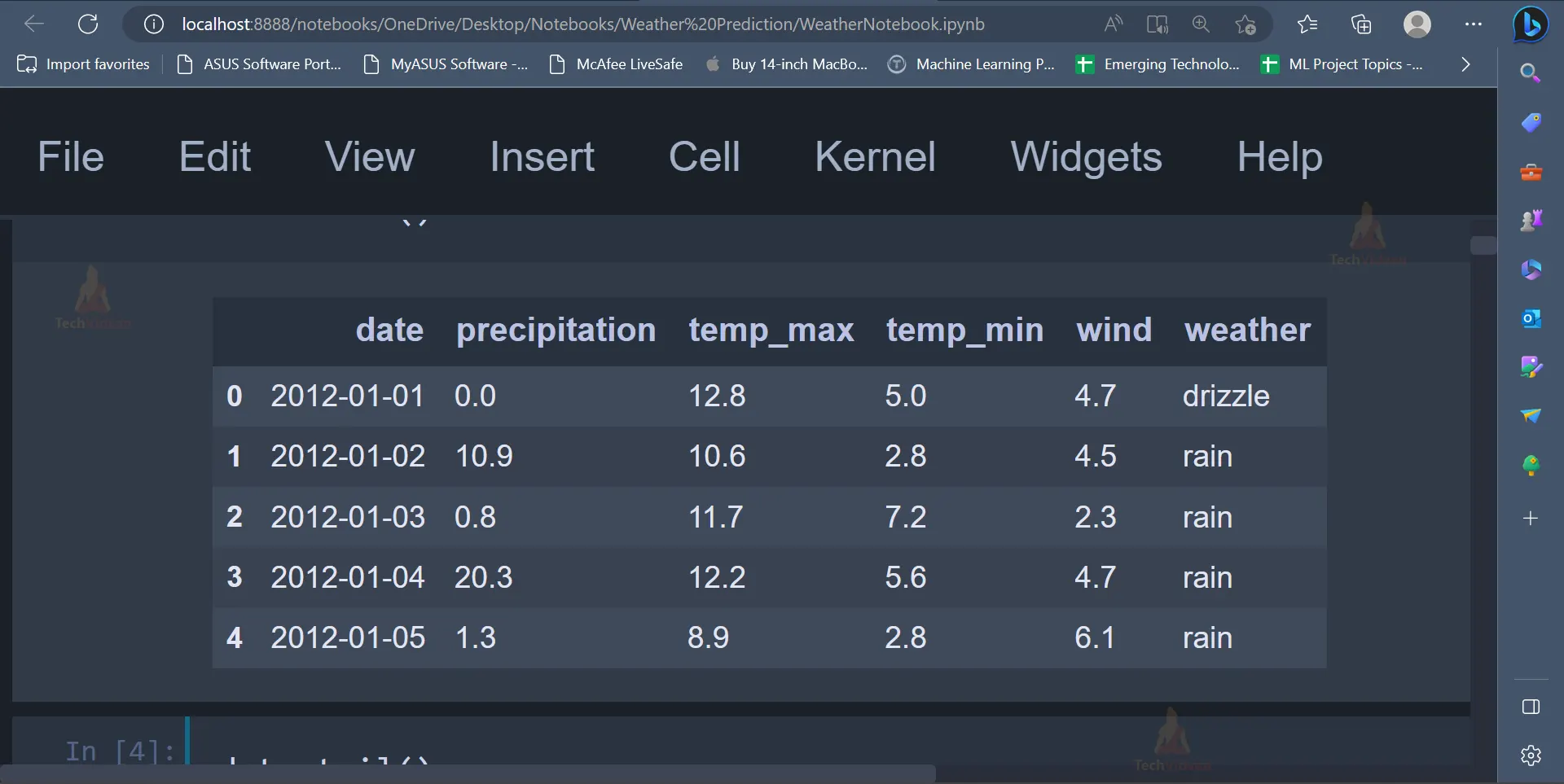
2. In the next step, the dataset is read using the read_csv() function and the first five rows of the dataset can be displayed.
#Load the dataset
data = pd.read_csv("weather.csv")
data.head()
Output
The output image displays the first five rows of the dataset.
3. Once the dataset is read and displayed, various exploratory data analysis techniques can be implemented on the dataset to gain more insights about the dataset.
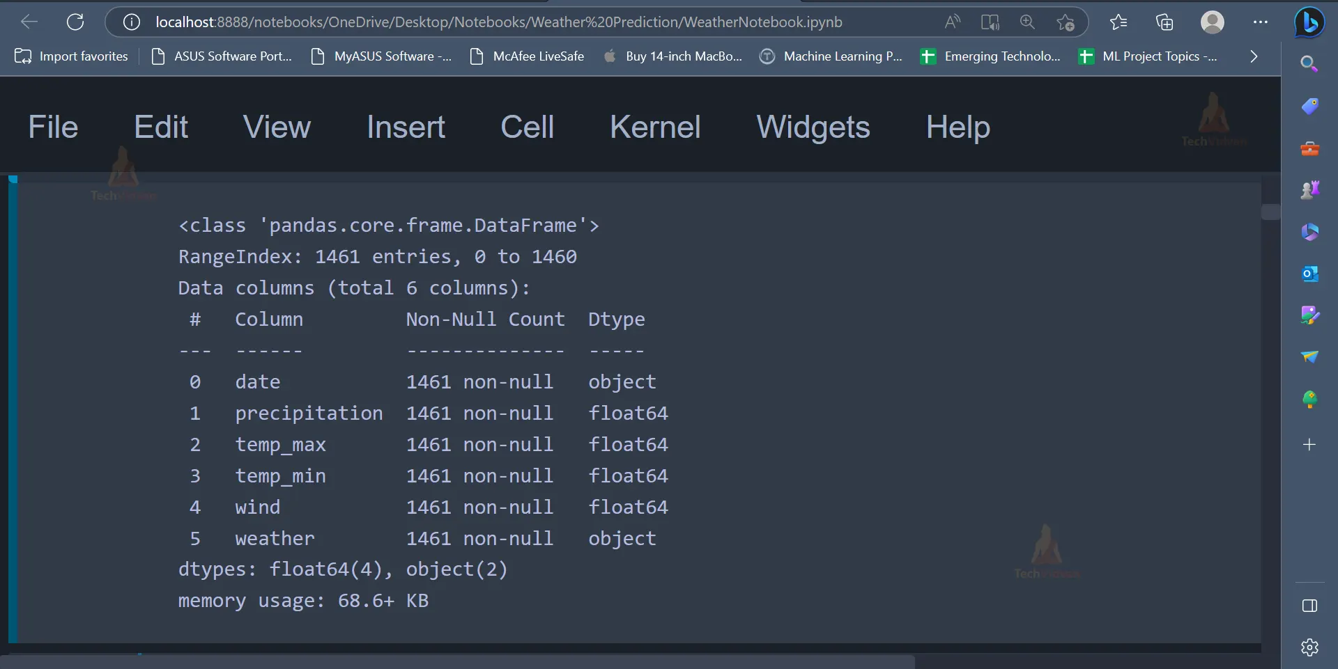
data.info()
Output
The info() function is used to display the number of rows and columns present in the dataset, the number of non-null values and the data type of all the attributes present in the dataset. The dataset contains 1461 rows and 6 columns.
4. Another way to check if there are any null values present in the dataset is to use the
isnull() function. The sum() function can be used along with the isnull() function to get the sum of null values in all the attributes.
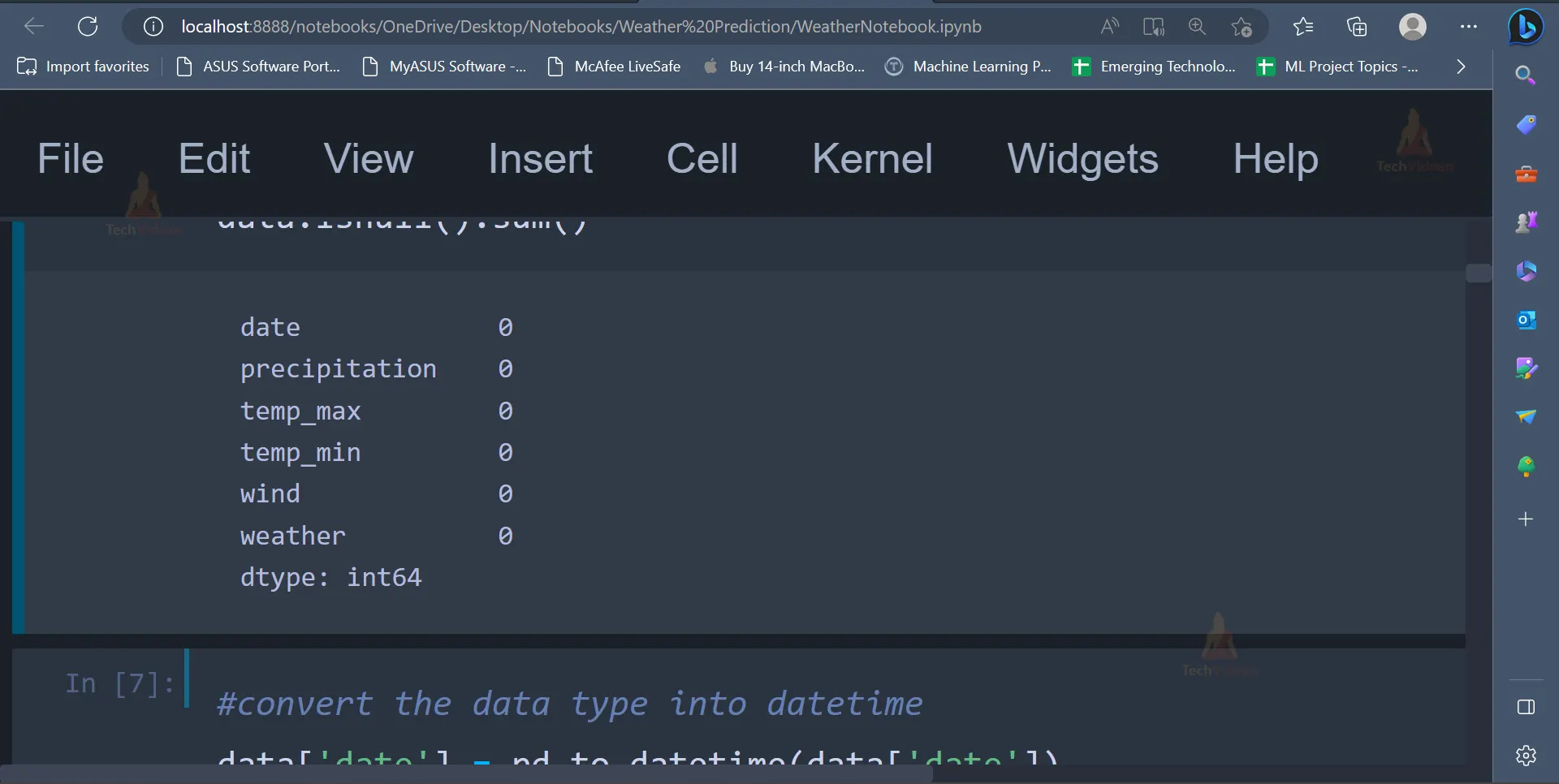
#Check for null values
data.isnull().sum()
Output
The output contains 0 as the value for all the columns. This means that there are no null values in any of the columns.
5. In the next step, the values present in the date column will be converted into date time format using the Pandas to_datetime() function.
#convert the data type into datetime
data['date'] = pd.to_datetime(data['date'])
6. After exploring the dataset, data visualisation techniques can be implemented to represent the data using graphs and charts.
plt.figure(figsize=(10,5))
sns.set_theme()
sns.countplot(x = 'weather',data = data,palette="ch:start=.2,rot=-.3")
plt.xlabel("weather",fontweight='bold',size=13)
plt.ylabel("Count",fontweight='bold',size=13)
plt.show()
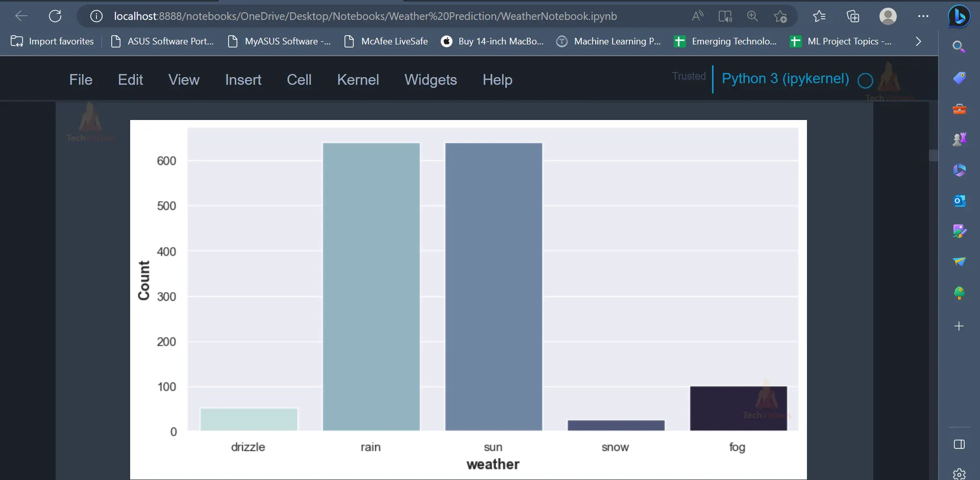
Output
The output displays the values present in the weather column using a countplot. It can be seen that the values rain and sun have the highest number of occurrences, and the value snow has the least occurrence.
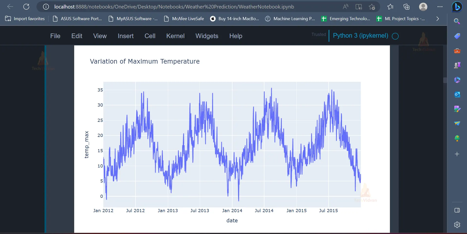
The line chart can be used to display the variation in maximum temperature on different dates.
px.line(data_frame = data,
       x = 'date',
       y = 'temp_max',
       title = 'Variation of Maximum Temperature')
Output
Since the graph is made using Plotly, the graph can be zoomed in and zoomed out to find out more details or to gain more insights. The same line chart can be implemented for values present in other columns as well.
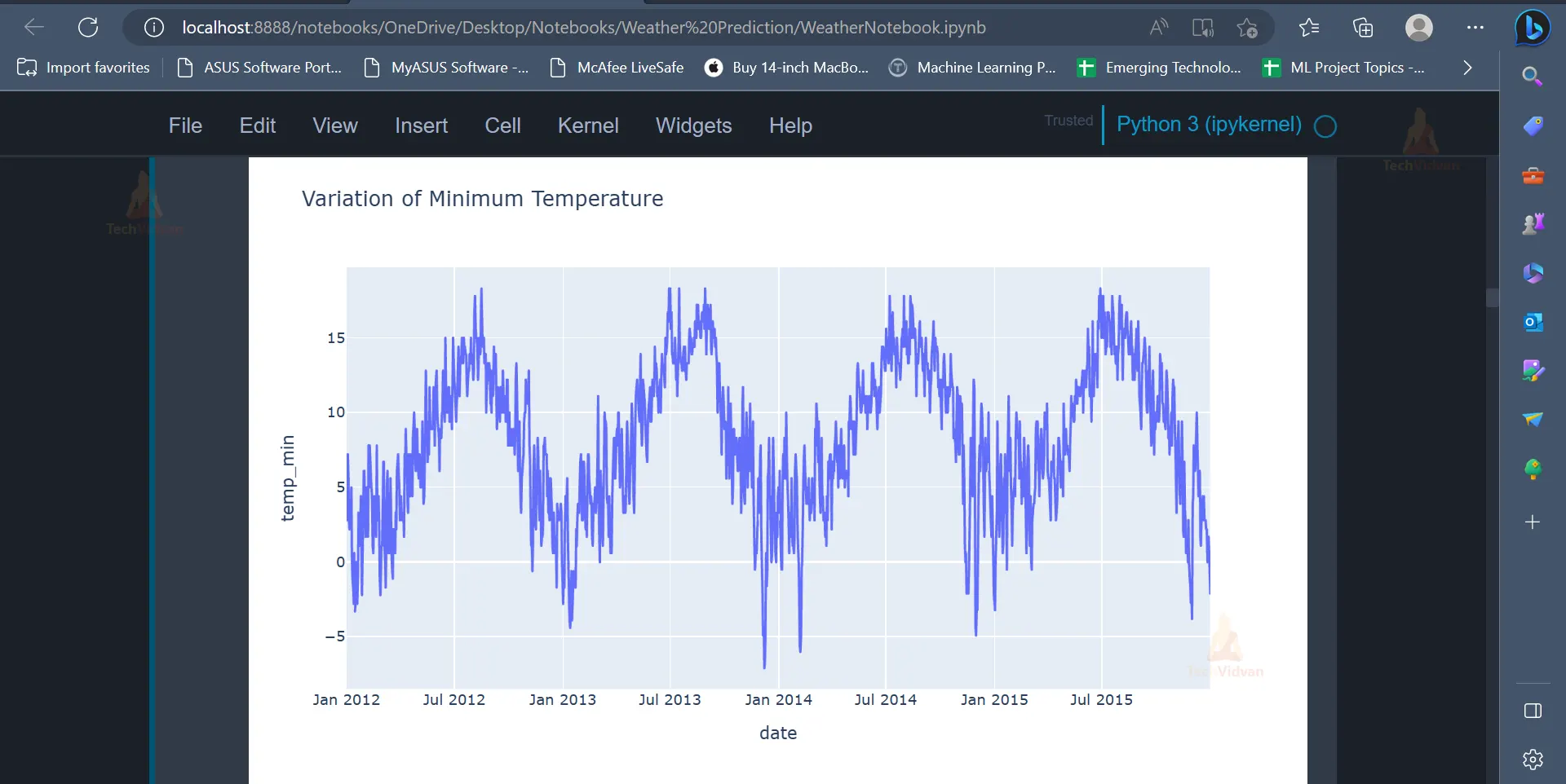
px.line(data_frame = data,
       x = 'date',
       y = 'temp_min',
       title = 'Variation of Minimum Temperature')
Output
Similar to the previous figure, the below output displays the variation of minimum temperature on different dates.
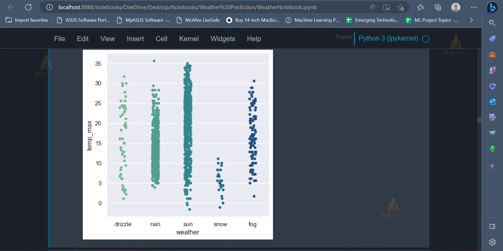
7. Catplot is a shorthand for categorical plots, which can be implemented to analyse the relationship between variables. The catplot provides the ability to create different categorical plots.
plt.figure(figsize=(10,5))
sns.catplot(x='weather',y ='temp_max',data=data,palette="crest")
plt.show()
Output
The output displays the relationship between the categorical variable(weather) and the numeric variable(maximum temperature). Each data point is represented by a scatter point, and the categorical factors decide how the scatter points are coloured and organised.
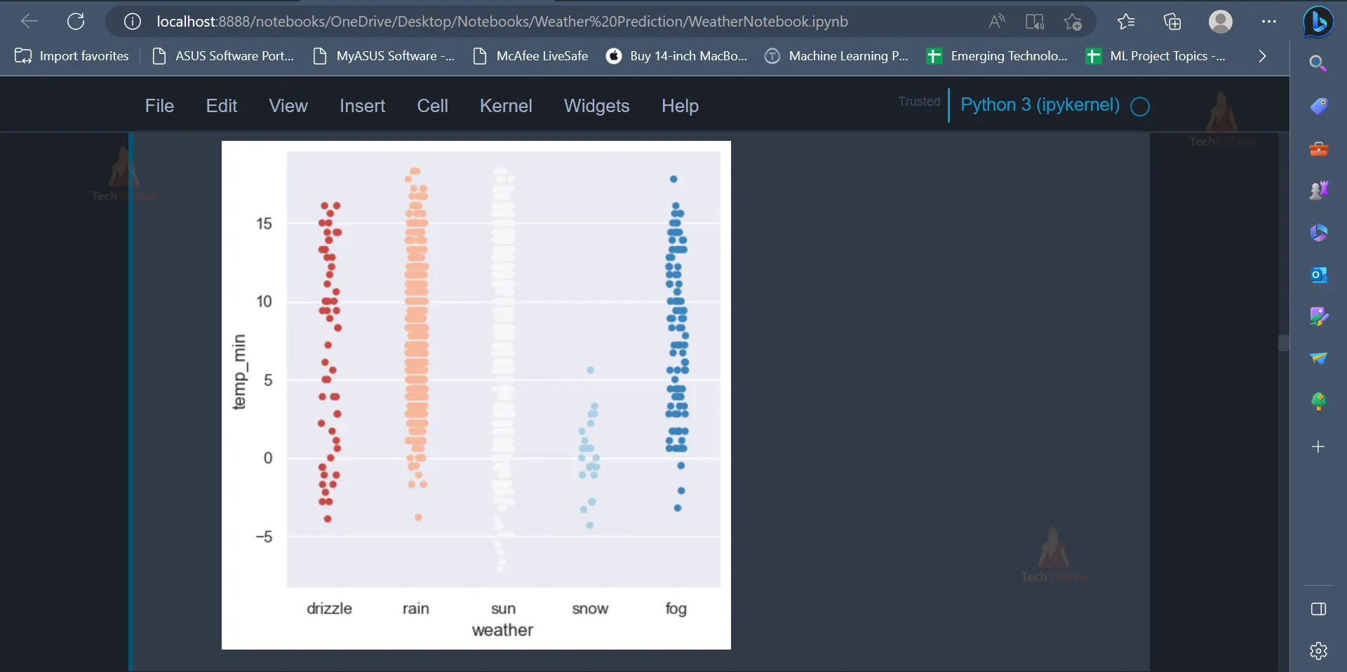
plt.figure(figsize=(10,5))
sns.catplot(x='weather',y ='temp_min',data=data,palette = "RdBu")
plt.show()
Output
The output contains the catplot for the weather column and the temp_min column.
8. Following data visualisation, the data can be pre-processed to convert the data into a form which can be better understood by Machine Learning models. We define a function called LABEL_ENCODING which can be used to convert categorical values into numerical values where in each categorical value is assigned with a unique integer value. We use this concept to convert the values in the weather column into integer values.
def LABEL_ENCODING(c1):
    from sklearn import preprocessing
    label_encoder = preprocessing.LabelEncoder()
    data[c1]= label_encoder.fit_transform(data[c1])
    data[c1].unique()
LABEL_ENCODING("weather")
9. Since the date column does not have any significance in the weather prediction, this column can be removed from the dataframe.
data = data.drop('date',axis=1)
10. After preprocessing the data, it can be split into independent variables(X) and dependent variables(y) using the below code.
x = data.drop('weather',axis=1)
y = data['weather']
All attributes except weather are independent variables/ independent attributes while weather is a dependent attribute.
11. It is important to split the dataset into training data and testing data, which can be later used to train the models and evaluate various models’ performance, respectively.
from sklearn.model_selection import train_test_split
X_train, X_test, y_train, y_test = train_test_split(x, y, test_size = 0.25, random_state = 0)
75% of the data is considered training data, and 25% of the data is considered testing data/test data.
12. Before we go ahead and start training Machine Learning models using the training data, we will make use of StandardScaler, which is an in-built sklearn preprocessing technique. It is a common method used in machine learning to normalise numerical data before feeding it into models that require standardisation.
from sklearn.preprocessing import StandardScaler
sc = StandardScaler()
X_train = sc.fit_transform(X_train)
X_test = sc.transform(X_test)
13. The first model which will be trained on the dataset would be Logistic Regression.
from sklearn.linear_model import LogisticRegression
classifier = LogisticRegression(random_state = 0)
classifier.fit(X_train, y_train)
Predictions from the Logistic Regression model can be made using the predict() function.
y_pred = classifier.predict(X_test)
The performance of models can be evaluated using metrics like confusion matrix, accuracy score etc.
sns.heatmap(cm,annot=True, fmt = '.3g')
acc1 = accuracy_score(y_test, y_pred)
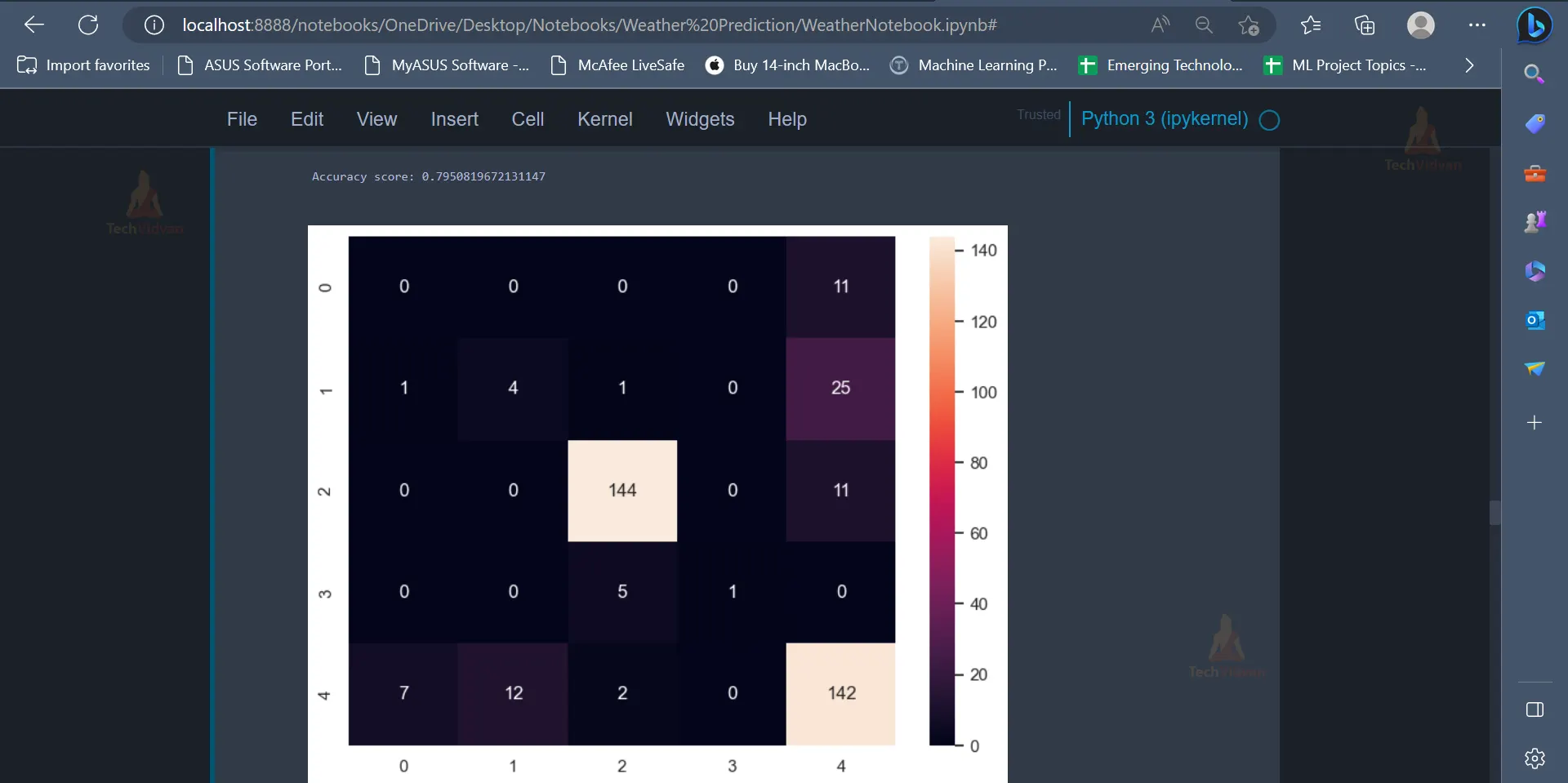
print(f"Accuracy score: {acc1}")
plt.show()

The values present in the diagonal of the confusion matrix (0,4,144,1,142) represent the number of data points which have been correctly classified by the model. From the accuracy score, it is evident that the model has an accuracy of 79.5%.
14. The next algorithm which will be used is the Naive Bayes Classifier.
from sklearn.naive_bayes import GaussianNB
classifier = GaussianNB()
classifier.fit(X_train, y_train)
The predictions are made in a way similar to how it was made earlier.
y_pred = classifier.predict(X_test)
cm = confusion_matrix(y_test, y_pred)
sns.heatmap(cm, annot = True, fmt = '.3g')
acc = accuracy_score(y_test, y_pred)
print(f"Accuracy score : {acc}")
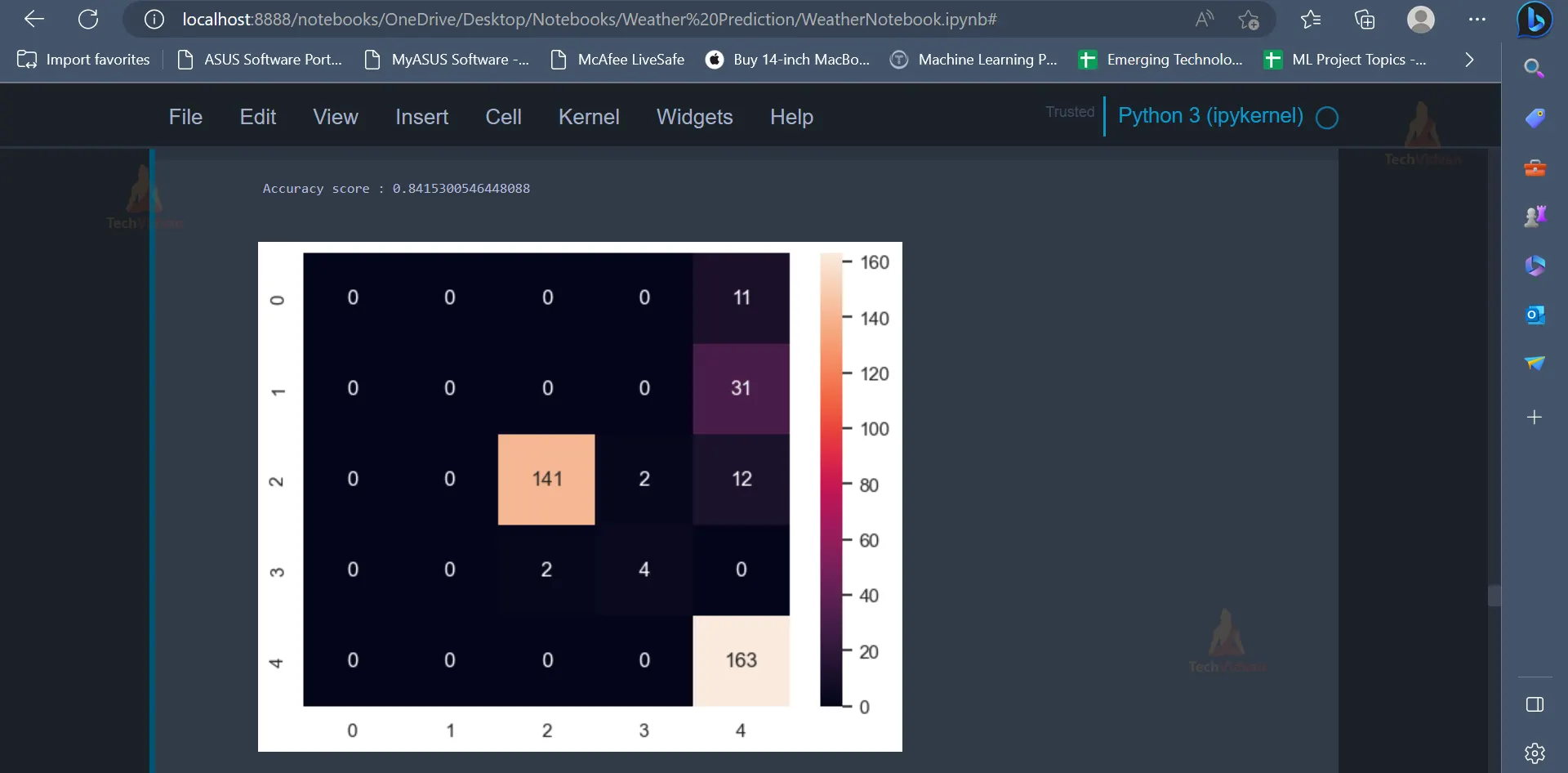
The Naive Bayes Classifier has an accuracy of 84.15%.
15. The last model which will be trained on the dataset would be the Support Vector Classifier.
from sklearn.svm import SVC
classifier = SVC(kernel = 'linear', random_state = 0)
classifier.fit(X_train, y_train)
y_pred = classifier.predict(X_test)
The confusion matrix and accuracy score can be displayed like earlier.
cm = confusion_matrix(y_test, y_pred)
sns.heatmap(cm, annot = True, fmt = '0.3g')
print(accuracy_score(y_test, y_pred))
The Support Vector Classifier provides an accuracy of 79.5 % on the dataset.
Conclusion
In conclusion, the project demonstrates the potential of machine learning in improving weather forecasting, aiding in decision-making processes, and assisting in various sectors such as agriculture, transportation, and emergency preparedness. While further research and improvements are necessary, this project highlights the significant potential of machine learning in enhancing weather prediction capabilities and advancing our understanding of atmospheric phenomena.