PCA and Factor Analysis in R – Methods, Functions, Datasets
In this TechVidvan tutorial, we will learn about principal component analysis (PCA) and factor analysis in R. We will learn what these techniques are and where they are used. Finally, we will implement them in R on a sample dataset.
Introduction to PCA and Factor Analysis
Principal component analysis(PCA) and factor analysis in R are statistical analysis techniques also known as multivariate analysis techniques. These techniques are most useful in R when the available data has too many variables to be feasibly analyzed. They reduce the number of variables that need to be processed without compromising the information conveyed by them.
What is Principal-Component Analysis?
Principal-component analysis (PCA) is a multivariate analysis technique. The basic idea behind this technique is to find variables with strong correlations between them and extract a single variable that can then represent them at the same time.
What are Principal-Components?
In the PCA, we find the correlation between all the available variables. We do this by making the covariance matrix of the dataset. Then we extract new variables that can depict the original information more efficiently than the older variables. We call these new variables as principal-components.
Our goal is to keep the number of principal-components less than the number of original variables. Thus, reducing the number of variables, we need to process.
Principal components are normalized linear combinations of the original variables. Let’s say that we have variable x1, x2, …,xn. Then our first principal component will be:
Z1=Φ11X1+Φ21X2+Φ31X3+…. +Φn1Xn
Where Z1 is the first principal component,
Φp1 is the loading vector of the first principal component. The loadings’ sum of squares is equal to one,
And X1, X2,…, Xn are normalized variables.
When do we use Principal-Component Analysis?
Imagine we need to predict the annual profits of a company in the year 2019. Assuming that we have the profits in the first quarter of 2019, the number of staff working in the company, their salaries, and the details of other expenditure by the company.
We can use other information such as tax reports, costs of ongoing ventures, and their expected returns. We also have the annual profits of the years 2018, 2017, 2016, and so on. It might look like we have a lot of variables to go on and make a prediction as accurate as possible. But that is where the problem lies.
We have a lot of variables.
PCA becomes useful in such cases. By finding variables with high correlation and grouping them, principal-component analysis reduces the number of variables we need to process without compromising the information they convey.
How does Principal-Component Analysis Work?
Here is a step-by-step overview of the process involved in principal-component analysis:
- Subtract the mean of every variable from each instance of them. Suppose we have m instances of n variables named A, B, and C, we would have a m x n matrix. Let’s call this matrix M.
- Find the covariance matrix of M. Let’s call this as CM.
- Compute the eigenvectors and eigenvalues of CM.
- Arrange the eigenvectors according to their eigenvalues.
- Select the eigenvectors with the highest eigenvalues. If we select k eigenvectors, we will get an n x k matrix. Let’s call this matrix EM.
- Obtain the transformed data. We can get the transformed data by using the following formula:
M’ = M*EM
Methods for Principal Component Analysis
There are two methods for principal component analysis. These are:
- Spectral decomposition
- Singular value decomposition
1. Spectral Decomposition
The spectral decomposition of a square m x m matrix A is defined as
A = UΔUT
Where U is an orthogonal matrix that is UUT=I, the columns of U are the eigenvectors of A,
And Δ is a diagonal matrix with A’s eigenvalues at it’s diagonal.
We can find a matrix’s principal components by performing spectral decomposition on its covariance matrix.
Don’t know much about R matrix? Learn to create, modify, and access R matrix components.
2. Singular Value Decomposition
The single value decomposition of an n x m matrix B, where n ≥ m, is defined as
B=UΓVT
Where U is an n x m orthogonal matrix, Γ is an m x m orthogonal matrix, and V is an n x n diagonal matrix. Here, the columns of Γ are the eigenvectors of B, and the square of the elements of the diagonal matrix V are the eigenvalues of U.
The singular value decomposition of the covariance matrix is another way of finding the principal components of a matrix.
Implementation of PCA in R
Now we will perform principal-component analysis on a dataset in the R programming language.
Performing PCA on a dataset
We will use the built-in dataset mtcars. The dataset has 32 instances for 11 variables. It gives 11 features like ‘miles per gallon’, ‘number of cylinders’, ‘horsepower’, etc. of 32 different models of cars. In the dataset, there are two categorical variables.
First is ‘vs’ that shows whether the car’s engine is ‘v’ shaped (1) or not (0).
The second one is ‘am’ that shows whether the car has an automatic transmission (1) or manual (0).
We will have to ignore these two variables in the analysis as PCA is for numeric data and cannot deal with categorical variables.
We will compute the principal components using the prcomp() function to achieve this.
Code:
mtcars.pca<-prcomp(mtcars[,c(1:7,10,11)],center=TRUE, scale.=TRUE)
summary(mtcars.pca)
Output:
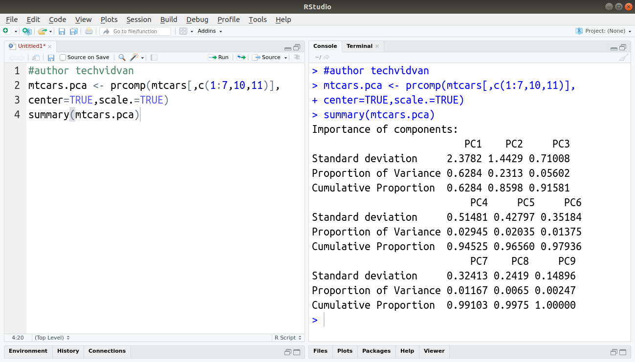
Viewing the results of PCA
The summary() function provides us with a summary of the object mtcars.pca, which stores the principal components extracted from the data. These components are arranged in decreasing order of importance. The proportion of variance shows us how much variation does a particular component covers.
As you can see, the first component PC1 covers almost 63% of the variance. If we use the second one as well, PC1 and PC2 represent almost 86% of the variance and, thus are sufficient to represent the original variables. As a result, we have reduced the 11 original variables to just two!
Plotting the results of the PCA
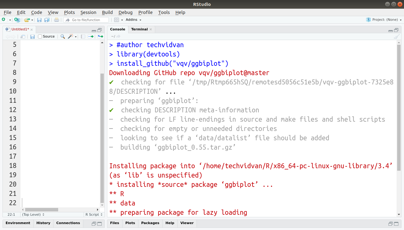
Now we will plot the PCA. We will be using a biplot, which shows the principal components as well as the old variables. To do that, we will be using the ggbiplot library. The ggbiplot package requires the devtools package, so make sure to install, and include that first.
Code:
install.packages(“devtools”)
library(devtools)
install.packages(“vqv/ggbiplot”)
Note: For R versions 3.4.4 and above, you can use the following command to install the ggbiplot package.
Code:
install_github(“vqv/ggbiplot”)
Output:
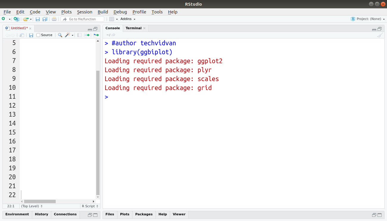
Once installed, include the package in the session by using the following command:
Code:
library(ggbiplot)
Output:
Now that the ggbiplot package is ready, we can use the ggbiplot() function to plot the principal components.
Code:
ggbiplot(mtcars.pca)
Output:
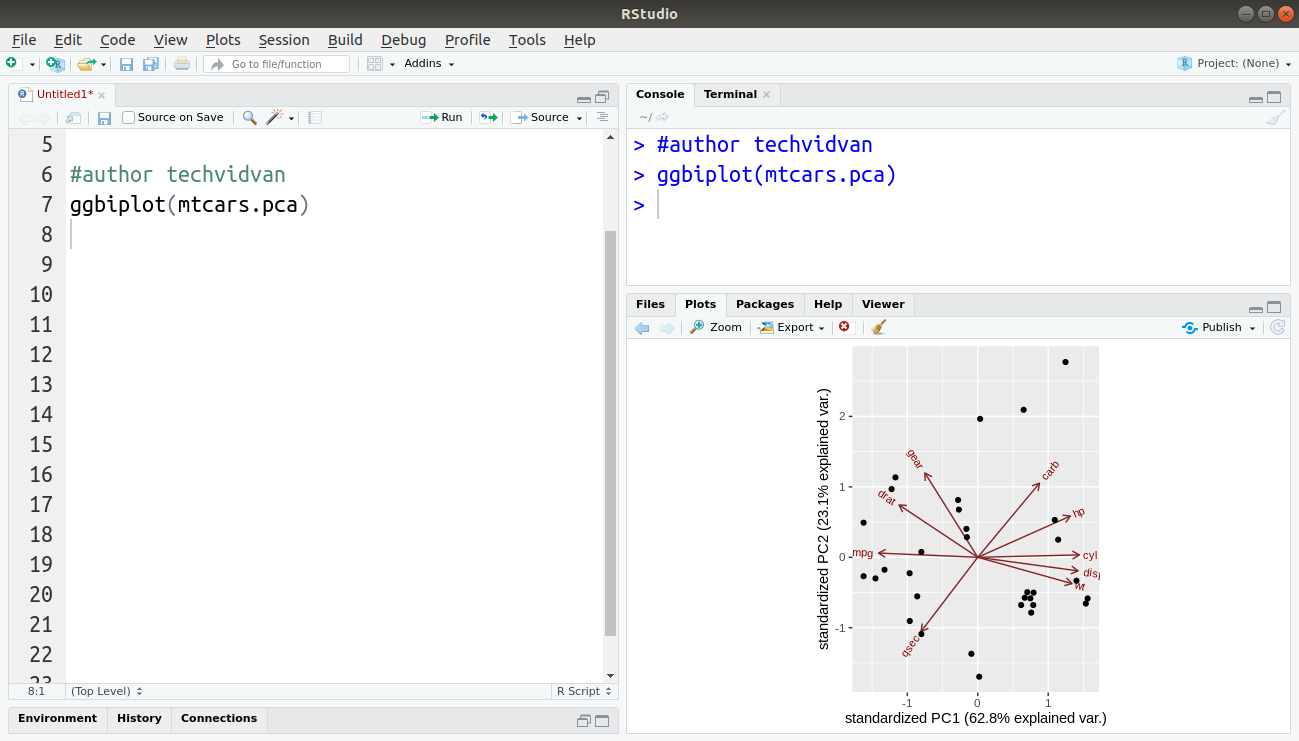
As you can see, we have successfully performed PCA on our dataset and plotted the results.
Factor analysis in R
Factor analysis (FA) or exploratory factor analysis is another technique to reduce the number of variables to a smaller set of factors. FA identifies the relationships among a set of variables and narrows it down to a smaller set.
We will be using the bfi dataset, which is a built-in dataset provided in R. It comprises 25 different personality factors. We will require the psych and the GPArotation packages. So, install and load them into the library. Then we will use the following command to find how many factors we need.
Code:
parallel <- fa.parallel(bfi,fm="minres",fa='fa')
Output:
Parallel analysis suggests that the number of factors = 7 and the number of components = NA

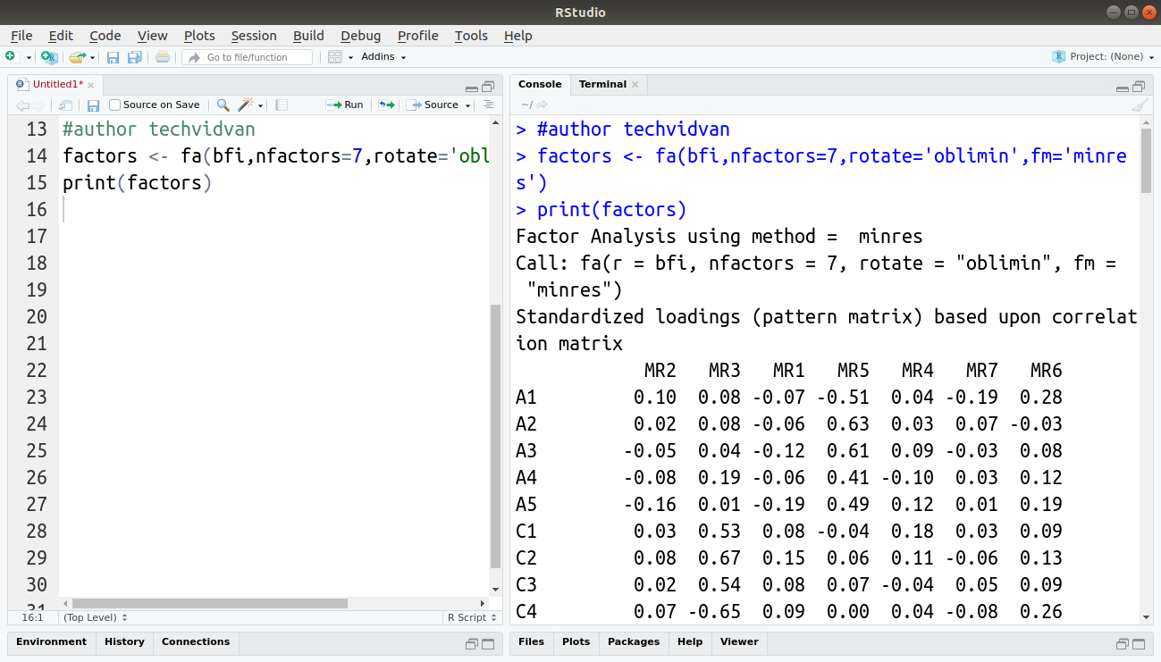
Now that we know how many factors we need, we can perform the factor analysis using the fa() function.
Code:
factors <- fa(bfi,nfactors=7,rotate='oblimin',fm='minres')
print(factors)
Output:
Summary
PCA and factor analysis in R are both multivariate analysis techniques. They both work by reducing the number of variables while maximizing the proportion of variance covered. The prime difference between the two methods is the new variables derived.
The principal components are normalized linear combinations of the original variables. The factors are measurement models of latent variables. While both techniques have the same purpose, they have different approaches and results.
In this tutorial, we learned what PCA and factor analysis are and also implemented the two techniques in R. We hope that this was an informative read to you.
Any difficulty while practicing PCA and factor analysis in R?
Ask our TechVidvan experts.
Keep Executing buddy!!