CNN in Tensorflow

Google built TensorFlow as the second machine learning framework that can be utilized to develop, create, and train deep learning models. The TensorFlow library was created due to numerical analyses which are done with data flow graphs. TensorFlow is a general deep learning framework. In this article, you will understand the basics of this Python library and comprehend how to execute these profound artificial neural networks with the help of it.

In this article we will be learning about the following topics:

1. What do you mean by Tensorflow and why is it necessary to use it in projects if python is used then you’ll be taught about tensors and how they vary from matrices.

2. Next you will be introduced to TensorFlow Framework, you will also see that using a computational diagram in TensorFlow, how a single line of code is executed.

3. Then you will understand some of the package’s notions that play a significant part in order for us to learn deep learning concepts like constants, variables.

4. Then, you’ll move on to the most fascinating domain of this tutorial which is the execution of the Convolutional Neural Network:

• You will attempt to comprehend the data.
• You’ll employ Python and its libraries to understand, use and study your data.
• You’ll also discover how to preprocess your data.
• You’ll understand how to envision your pictures as a matrix, reshape your data and rescale the pictures between 0 and 1 if required.

Tensors

A tensor is a way of displaying the data in deep learning.

A tensor can be a 1-dimensional, a 2-dimensional, a 3-dimensional array but we can think of a tensor as a multidimensional array.

The reason why we use machine learning and deep learning is that you have datasets that have very dimensional regions, in which per dimension denotes a further part of that dataset.

This can be understood in a better way if we understand the example of the features in a leopard and cheetah; here the dataset you’re performing with has numerous types of both leopard and cheetah pictures.

Now, in order to accurately categorize a leopard or a cheetah when shown an image, the network has to understand discriminatory components like color, ears, face structure, eyes, the length and shape of the tail, etc. These elements are included by the tensors.

The name “TensorFlow” is derived from the operations that neural networks perform on multidimensional data arrays or tensors! It’s literally a flow of tensors.

Familiarising Tensors

In order to understand tensors and why we use them it is good to have some working understanding of linear algebra and vector calculus. With more explanation, we can fully learn tensors and their help in machine learning.

Vectors and tensors are almost the same. The very most suitable way to comprehend tensors is to begin by making sure that you’re stable on your knowledge of vectors.

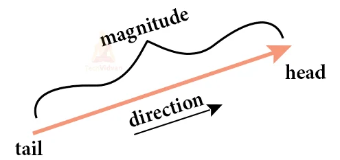
Vector is a quantity that has both magnitude and direction, where the measurement of the arrow is proportional to the magnitude of the quantity and the direction of the arrow tells you the direction of the quantity.

This could represent the force of gravity or the direction of the Earth’s magnetic field. Vectors can also symbolise other quantities as well, such as an area.

How does a vector illustrate an area?

The length of the vector is proportional to the portion of the area (the number of square metres in the area) and then you make the direction of the arrow perpendicular to the surface.

So in that way, this can illustrate an area as well. So vectors can represent lots of things. Vectors are components of a more expensive type of object called tensors.

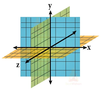
This represents a coordinate system – the x-axis, the y-axis, and the z-axis all meeting at right angles. This represents the Cartesian coordinate system, and they come along with coordinate basis vectors.

They are also referred to as “unit vectors” and have a length of one.

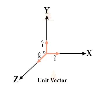
The direction of the basis vectors or unit vectors is in the direction of the coordinate axes, so this might illustrate the unit vector in the x-direction that’s often called “x” with an “i-hat”. That’s the x-hat unit vector – it indicates the direction of increasing x coordinate.

So since we have the coordinate system and the unit vectors in place, now we will be able to find the components of your vector.

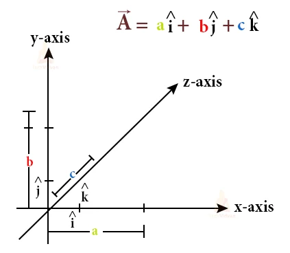
All these features can be used as a vector. We can represent it as an array. We can also represent them as a stack. These glimpses are just like the column vectors.

Because there’s an exclusively one basis vector per component. This is what causes vector tensors to be of rank one or one basis vector per component.

By the exact idea, scalars can also be tensors of rank zero, because scalars have no directional arrows, thus require no indices. Therefore those are tensors of rank zero.

 

This is an illustration of a rank-two tensor in three-dimensional space. So we can have nine elements and nine sets of two basis vectors.

Witness that the components do not have a single index, they have two indices.
Why might you need such an expression?

Consider a solid object and all the forces inside a box. Inside that object, we can imagine surfaces whose area vectors reveal in the x- or in the y- or in the z-direction.

And on each of those sorts of surfaces, there might be a force that has a component in the x- or in the y- or in the z-direction. So to completely represent all the potential forces on all the likely surfaces, we need nine components, each with two indices directing to basis vectors.

We can also have a mixture of nine components and nine sets of two basis vectors making this a rank-two tensor.

The miniature of a rank-three tensor in three-dimensional space: 27 components according to one of 27 sets of three basis vectors. It is about the mixture of components and basis vectors that makes tensors so powerful.

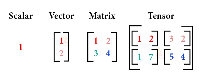
Vectors are unique kinds of matrices, which are rectangular arrays of numbers. Because vectors are collections of numbers, they are frequently seen as column matrices: they have just one column and a certain number of rows. In other terms, you could also think of vectors as scalar magnitudes that have been given a direction.

So what about plane vectors then?

Plane vectors are the most detailed setup of tensors. They are much like regular vectors, with the exclusive distinction that they discover themselves in a vector space.

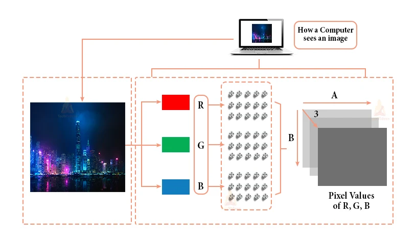
How does a computer read an image?

• The image can be broken down into 3 colour channels: Red, green, and blue.
• Each of these colour channels is mapped to the image’s pixel.
• Then, the computer recognizes the value in association with each pixel and finds the size of the image
• For black-white images, there is only one channel, and the concepts are the same.

What is CNN?

• Convolutional Neural Networks are like neural networks, are made up of neurons with given weights and biases. Each neuron after it receives information takes a weighted sum over them, gives it to an activation function, and responds with an output.
• The entire network has a loss function, and all the information and schemes that we developed for neural networks still involve Convolutional Neural Networks.
• Neural networks, as its name implies, are a machine learning approach that is modelled after the brain structure. It includes a network of learning units called neurons.
• These neurons comprehend how to convert input signals(e.g. image of a cat) into corresponding output signals(e.g. the label “cat”), including the foundation of automated recognition.

Let’s take the standard of automatic image recognition. The procedure of deciding whether a photo includes an act applies an activation function. If the picture reaches prior cat images the neurons have seen before, the label“cat” would be started.

How CNN works?

There are four layered ideas we should comprehend in Convolutional Neural Networks:

1. Convolution,

2. ReLu

3. Pooling and

4. Full Connectedness (Fully Connected Layer).

There are numerous renditions of X and O’s. This causes it to be tough for the computer to remember it. But the goal is that if the input signal looks like the last pictures it has visited before, the “image” reference signal will be incorporated into, or convolved with, the input signal. The resultant output signal is then handed on to the next layer.

So the computer comprehends every pixel. In this case, the white pixels are 1 and the black ones are 1. This is just the path we’ve executed to determine the pixels in a basic binary classification.

Presently if we would just generally search and approximate the values between a normal image and another version, we would get a lot of lost pixels.

We take miniature patches of the pixels called filters and try to check them in the corresponding nearby locations to see if we get a match. By doing this, the Convolutional Neural Network gets a lot more reasonable at noticing similarities than instantly trying to match the entire image.

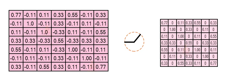
Convolution of an image

Convolution has the agreeable property of being translational invariant. Intuitively, this means that each convolution filter denotes a part of interest (e.g pixels in letters), and the Convolutional Neural Network algorithm knows which features include the consequent reference(i.e. alphabet).

Steps in regards to processing the image using CNN

ReluLayer

ReLU is an activation function.

What is an activation function?

Rectified Linear Unit(ReLU) transform function just activates a node if the information is above a specific amount, while the information is below zero, the outcome is zero, but when the input increases above a particular threshold, it has a linear association with the dependent variable.

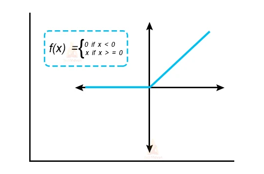
The primary purpose is to clear all the negative weights from the convolution. The positive values stay identical but all the negative values get modified to zero as indicated in the image:

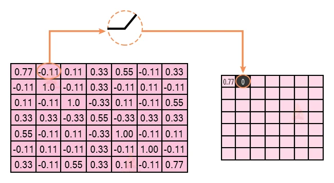
After the process, we get the following output:

Pooling layer

In this coating, we shrink the picture stack into a more diminutive size. Pooling is done after giving through the activation layer. We do this by executing the subsequent 4 stages:

• Pick window size(usually 2 or 3)
• Choose astride(usually 2)
• Step your window across your filtered pictures
• From each window, bring the highest importance

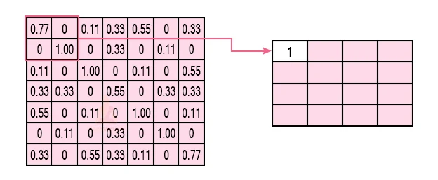
Pooling layer example

• Consider serving pooling with a window size of 2 and stride being 2 as well
• So in this case, we took the window size to be 2and we got 4values to choose from. From those 4 values, the maximum value there is 1. In that case, we choose 1.

Note that we created out with a 7×7matrix but currently the exact matrix after pooling reached down to4×4

But we ought to carry the window across the real picture. The process is precisely as exact as above and we ought to replicate that for the full picture.

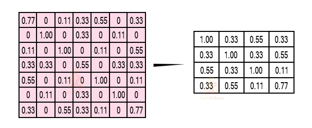
So to get the time-frame in one picture we’re here with a 4×4matrix from a7×7matrix after giving the input through 3 layers –Convolution, ReLU, and pooling and after the double pass we get a 2 × 2 matrix as shown in the image:

Next step

• The final layers in the network are fully related, suggesting that neurons of preceding layers are related to every neuron in succeeding layers
• This mimics high-level reasoning of evaluation of all potential pathways from input to output.
• Also, the fully connected layer is the final layer where the category really occurs. Here we bring our filtered and shrunk pictures and put them into one single list as displayed :

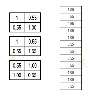Also, the fully connected layer is the final layer where the classification actually happens. Here we take our filtered and shrunk images and put them into one single list as shown above.

when we provide in, ‘X’ and ‘O’ there will be some element in the vector that will be increased.

Imagine the picture down, as you can see for ‘X’ there are additional features that are high and also, for ‘O’ we have additional features that are high

When the 1st, 4th, 5th, 10th, and 11th values are increased, we can organize the image as ‘x’. The idea is identical for the different alphabets as well –when specific values are placed the way they are, they can be mapped to an existing letter or a numeral which we require

Tensorflow Implementation using CNN.

Now, let’s look at the implementation, training, and evaluation of the Convolutional neural network.
Let’s discuss this in three steps

Step 1 – Compile the CNN model

Step 2 – Fit model on the training set

Step 3 – Evaluate the Result

Lets implement the above steps one by one

Step 1 – Compile CNN Model

Code line-

model.compile(loss=’categorical_crossentropy’,optimizer=’adam’,metrics=[‘accuracy’])

Here we are utilizing 3 opinions:-

• Loss function

We are utilizing the categorical_crossentropy loss function that is employed in the classification task. This loss is an extremely useful step of how different two discrete probability distributions exist from each other.

• Optimizer

We are employing adam Optimizer which is utilized to edit neural network weights and understanding rate. Optimizers are employed to translate optimization issues by minimizing the function.

• Metrics arguments

Here, we are utilizing Accuracy as a metric to estimate the implementation of the Convolutional neural network algorithm.

Step 2 – Fit Model on the Training Set

Code Line:

model.fit_generator(training_set,validation_data=test_set,epochs=50, steps_per_epoch=len(training_set), validation_steps=len(test_set) )

Here we fit the CNN model on the training dataset with 50 iterations and each iteration has various measures for training and assessing steps founded on the measurement of the test and training set.

Step3:- Evaluate the Result

We reach the accuracy and loss function for both the training and test dataset.

Code: Plotting the loss graph

plt.plot(r.history['loss'], label='train loss')
plt.plot(r.history['val_loss'], label='val loss')
plt.legend()
plt.show()
plt.savefig('LossVal_loss')

Output:

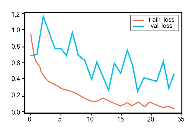
Loss is the penalty for a bad projection. The purpose is to make the validation failure as low as feasible. Some overfitting is nearly invariably the right thing. All that concerns, in the end, is: is the validation loss as low as you can obtain it.

Code: Plotting the Accuracy graph

plt.plot(r.history['accuracy'], label='train acc')
plt.plot(r.history['val_accuracy'], label='val acc')
plt.legend()
plt.show()
plt.save
fig('AccVal_acc')

Output:

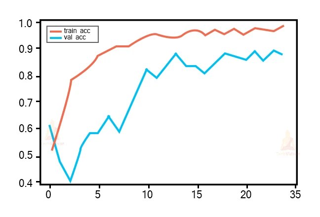
Accuracy is one metric for assessing classification models. Informally, accuracy is the trace of predictions our model got good. Here, we can keep that accuracy inches toward 90% on validating test which denotes a CNN model performs well on accuracy metrics.

Let’s look at another implementation where we will be using Fashion-MNIST dataset

Fashion-MNIST Dataset

We will be looking into Fashion-MNIST. The Fashion-MNIST dataset includes Zalando’s article images, which contains 28×28 grayscale pictures of 65,000 fashion products from 10 categories, and 6,500 photographs per category. The training collection has 55,000 images, and the test set has 10,000 images.

It is used to categorize handwritten digits. That suggests that the image measurements, movement, and test splits are similar.

You can locate the Fashion-MNIST dataset online.

To load the data, you preferably must download the data set, and then you will be able to perform with it.

Load the data

You first start with importing all the libraries like NumPy, Matplotlib, and, most importantly, Tensorflow.

For clarity, let’s construct a dictionary that will have class terms with their related absolute class labels.
Also, let’s take a peek at a pair of photos in the dataset:

Data Preprocessing

The photos are of a 784-dimensional vector. The pictures are already rescaled between 0 and 1, so you don’t require to rescale them likewise, but to be certain, let’s imagine a picture from the training dataset as a matrix.

The dataset has class labels,

0 –T-shirt/top

1 –Trouser
…
9 –Ankle Boot

Given in pictures, we ought to organise them into one of these classes, hence, it is basically a‘ Multi-class Classification’ problem.

How to visualize a deep learning model?

The fastest path to visualize your model is to use the model summary function.

Compiling the Model

Compile tells us about the loss function, the optimizer, and the metrics. We can also use fit() for training the model with the provided inputs and corresponding training labels.

We need not reshape the labels because they already have the correct dimensions. We can also check the predicted and correct values of our mode.

Classification report

Gives us information about the F-1 score.
The F1 score is a weighted harmonic standard of precision and recollects such that the most useful score is 1.0 and the imperfect is 0.0. F1 scores are lower than accuracy measures as they entrench precision and identify into their computation.

Finally, we can save our model using model.save().

Summary

In this article, you have realized CNNs from their concepts to their applications in the natural world. We have also witnessed that you can use current architectures to quicken your model growth method. Particularly, we have learned that:

• What are convolutional neural networks
• How convolutional neural networks function
• What are vectors and tensors
• How are tensors used to process and train images
• Utilizing pre-trained convolutional neural networks using Fashion MNIST
• Creating convolutional neural networks from scrape using TensorFlow
• Saving your best model
• Classification report

TensorFlow delivers pre-built processes and progressive operations to facilitate the job of creating various neural network models. It delivers the needed infrastructure and hardware which makes them one of the most significant libraries used considerably by students and experts in deep learning.