Data Structures Asymptotic Analysis
In this article, we are going to learn about the concept of asymptotic analysis and various asymptotic notations used for the analysis of any algorithm.
Defining asymptotic analysis
Whenever we write an algorithm for a particular computational problem, we design the algorithm in such a way that it gives the best results in terms of running time as well as memory used.
While checking the running time for any algorithm, we want three things:
1. The algorithm should be machine-independent.
2. It should work on all possible inputs.
3. It should be general and not programming language-specific.
However, we never do accurate analysis, rather we do approximate analysis. We are interested in the increase in the running time with the increase in the input size. Thus, we are only interested in the ‘growth of the function’, which we can measure/analyse through asymptotic analysis.
1. Asymptotic analysis is a general methodology to compare or to find the efficiency of any algorithm.
2. We measure the efficiency in terms of the growth of the function. The growth of any function depends on how much the running time is increasing with the increase in the size of the input.
Assumptions for Asymptotic Analysis
Asymptotic analysis is based upon certain assumptions such as:
Let Rt be the running time of an algorithm, N be the input size. Then,
1. Rt ≥ 0 and N≥0 i.e. both running time and input size should be positive numbers.
2. The input size is very large while analyzing any algorithm through asymptotic analysis i.e. N→∞
3. The analysis is both hardware independent and software independent.
4. For better understanding, we do a high-level representation of the algorithm i.e. pseudo-code or English like instructions.
5. We focus on primitive operations i.e. those operations which are independent of software such as assignment, comparison, arithmetic operations, etc in terms of input size.
Example:
Let us try to get a brief idea behind the concept of asymptotic analysis with the help of an example.
1. Suppose we wish to calculate the value of 1 + 2 + 3+ 4+ —— + n
2. There could be two possible ways to do that.
3. One of the ways is to write the formula directly as shown:
int n, sum=0;
sum = (n * (n+1))/2;
4. Another way is iteratively finding the sum as shown:
int n, sum=0;
 for(i=1; i<=n; i++){
     sum = sum + i;
 }
5. In the first method, where we are using the direct formula, every time the number of steps is the same because, for whatever value of n, the formula will run in a single step.
6. Thus, we can say that method 1, where we are using the formula to find the sum, is taking constant time because it is completed in a constant number of steps.
7. However, in the 2nd method, the number of steps executed by the program will depend on the value of n because for loop is running n times.
8. This is why the number of steps in the 2nd method is not constant but linearly dependent on n.
9. From here, we can conclude that the computation time taken by the second method is more than the first method.
This is the basis of our analysis.
How to find the time complexity?
1. It is not practically feasible to sit and calculate the time taken by an algorithm to run on a system.
2. However, we know that the running time of an algorithm depends on the size of the input. So, we can use this input size to analyse the time taken by an algorithm.
3. Let us again take the above example of finding the sum of first n natural numbers iteratively.
int n, sum=0;
    for(i=1; i<=n; i++){
        sum = sum + i;
    }
4. In this code, if the value of n is 10, the algorithm will take 10 units of time.
5. But for the same code, if the value of n is 1000, the algorithm will take 1000 units of time for execution.
6. Therefore, if the input is n, then the time complexity for any algorithm is a function of n, say T(n).
How to calculate the value of T(n)
1. Let T(n) be a function that denotes the time complexity for an algorithm.
2. Then, to find the value of T(n), we need to check for various values of n.
3. Usually, finding the value of T(n) for smaller problems is easy as compared to the larger ones.
4. For example, suppose a function is T(n) = 3n2 +5n + 8
5. Then for smaller values of n, such as for n=1,2,3,4….9, the value of T(n) depends on the whole equation.
6. However, whenever we do asymptotic analysis, we always consider n to be very large (as described in the assumptions).
7. For larger values of n i.e. n→∞, the value T(n) depends only on the highest power and hardly depends upon other values in the equation.
8. In the above example, for higher values of n, T(n) will come out to be T(n) = 3n2.
9. Usually, we discard the value of constant, which is 3 here.
10. So we can conclude that the value of T(n)=3n2 +5n + 8 is of the order of n2
Usually, there are three different categories depending on the time taken by an algorithm:
1. Worst case
It describes the scenario in which the algorithm takes the highest amount of time.
2. Best case
It describes the case in which the running time of the algorithm is minimum.
3. Average case
It lies between the best case and worst case. Precisely, it takes the average time that an algorithm will take to execute.
Asymptotic Notations
The three most commonly used notations for finding the running time or the time complexity of an algorithm are:
1. Big Oh notation(O)
2. Omega notation(Ω)
3. Theta notation(θ)
1. Big Oh notation(O)
a. This notation describes the upper bound of the running time for an algorithm.
b. Big Oh notation ensures that the function never grows faster than its upper bound.
c. Thus, it measures the performance of an algorithm by describing the order of growth for a function and by giving the least upper bound for that function.
d. Big Oh measures the worst-case time complexity for the given algorithm i.e., it measures the longest time an algorithm can execute.
Computing O(n)
a. Let there be two functions- f(n) and g(n) defined for positive integers as shown:
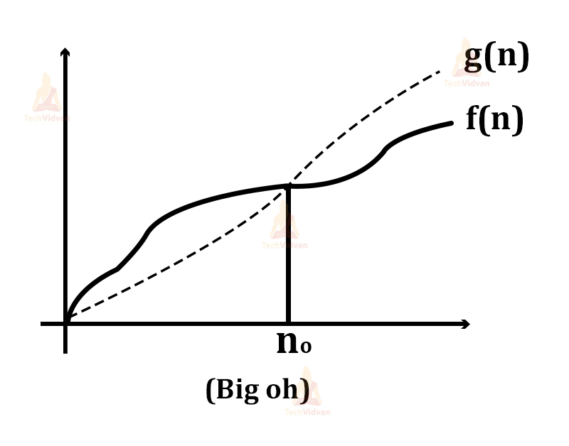
b. Then f(n) = O(g(n)) as growth of g(n) is faster than that of f(n).
c. f(n) = O(g(n)) is read as f(n) is equal to Big Oh of g(n).
d. Mathematically, we can say that f(n) ≤ c.g(n) for constants c and n0 where c>0 and n>n0.
e. This implies that the function g(n) is an upper bound on the function f(n) i.e. f(n) cannot grow faster than g(n).
Let us try to understand this concept with the help of an example:
For Example:
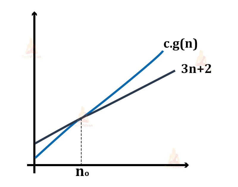
1. Let f(n) = 3n+2 and g(n) = n. We need to check whether f(n) = O(g(n)) or not.
2. For f(n) to be equal to O(g(n)), both the functions f(n) and g(n) must satisfy the following condition: f(n) ≤ c.g(n).
3. To check if the condition holds, replace f(n) by 3n+2 and g(n) by n i.e. 3n+2 <= c.n
4. Let c=7 and n=1, then 3(1)+2 <= 7*1 ⇒ 5<=7 which is true.
Thus, f(n) <= c.g(n) is true for n=1.
5. For n=2,
3(2)+2 <= 7*2 ⇒ 8 <= 14 which is again true.
6. Therefore, f(n) <=c.g(n) is true for n=2 as well.
7. From here, we can conclude that f(n) <= c.g(n) holds for all values of n, given that c=7.
8. Thus, we can say that the above equation always holds for some constant c and some constant n0.
9. So, f(n) is equal to Big Oh of g(n) i.e. f(n) = O(g(n)) or we can say that c.g(n) is an upper bound on function f(n).
Big Oh notation always gives the worst-case time complexity for a function or algorithm as it is based on comparison with the upper bound of a function.
2. Omega notation(Ω)
1. It is the opposite of Big-Oh notation.
2. Omega notation always describes the best-case scenario for a particular algorithm.
3. Omega represents the lower bound of running time for an algorithm.
4. It will measure the least amount of time that an algorithm can take for its execution in the best case.
Computing omega:
1. Let f(n) and g(n) be two functions defined on a set of natural numbers.
2. Then, f(n) = Ω(g(n)) only if the growth of f(n) is faster than the growth of g(n).
3. Mathematically, its equation will be f(n) ≥ c.g(n) where c and n0 are constants such that c>0 and n>n0.
Let us understand this notation with the help of an example:
1. Let f(n) = 2n+3, g(n) = n, we need to find whether f(n)= Ω (g(n)) or not.
2. For f(n) to be equal to the omega of g(n), it must satisfy the condition: f(n)≥ c.g(n)
3. Replace f(n) by 2n+3 and g(n) by n 2n+3 ≥ c*n
4. Let c=1 i.e. value of constant c=1.
5. For n=1,
2(1) + 3 ≥ 1(1) .⇒ 5 ≥ 1 which is true.
6. Similarly, for n=2,
2(2)+3 ≥ 1(2) ⇒ 7 ≥ 2 which is again true.
7. If we check for further values, the equation holds for every value of n given that c=1.
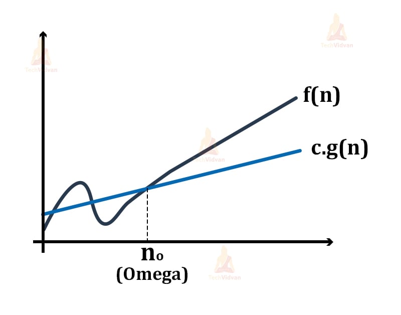
Here, the function g(n) is the lower bound of the function f(n) and thus it gives the running time for the function f(n) in the best possible case.
3. Theta notation(Θ)
1. While Big Oh gives the worst-case analysis and omega gives the best case analysis, theta lies somewhere in between.
2. Theta notation gives the average case analysis for a function or algorithm.
3. In real-world problems, not every time the algorithm will have either the best or worst-case scenario.
4. Practically, an algorithm is always performing in some average case i.e. the algorithm keeps on fluctuating.
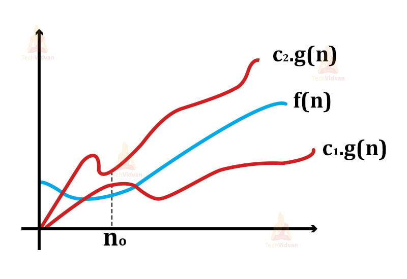
Computing Theta
1. Let there be two functions: f(n) and g(n) defined on a set of positive integers.
2. Then, f(n) = Θ(g(n)) if
c1.g(n)≤ f(n)≤ c2.g(n) where c1, c2 are constants.
3. In theta notation, two limits bind the function i.e. both the upper limit as well as the lower limit. This is what makes the theta notation return the average case for an algorithm.
4. Thus, the condition f(n)= θg(n) becomes true only when c1.g(n) is less than or equal to f(n) and c2.g(n) is greater than or equal to f(n).
Let us understand the Theta notation with the help of an example:
1. Let f(n) = 2n+3 and g(n) = n.
2. Replace f(n) with 2n+3 and g(n) with n in the equation c1.g(n)≤ f(n)≤ c2.g(n).
Then the equation will be c1.n ≤2n+3≤ c2.n
3. To ensure that the equation holds, let c1=1 and c2=5.
4. Thus, for n=1,
the equation will be 1(1) ≤ 2(1)+3 ≤ 5(1) ⇒ 1 ≤ 5 ≤ 5 which is true.
5. For n=2,
The equation will be 1(2) ≤ 2(2)+3 ≤ 5(2) ⇒ 2 ≤ 7 ≤ 10 which is again true.
6. Hence, we can say that the equation holds for all the values of n given that c1=1 and c2=5.
7. Therefore, we can say that for the above example, f(n) is equal to θ(g(n)). And it gives average-case complexity for f(n).
Example:
Let us consider the following example for more understanding:
Assume we have to reverse the string: “TechVidvan”. The traditional algorithm for it is:
1: START
2: Declare two variables str1 and str2.
3: Initialize the variable str1 with “TechVidvan”
4: Traverse to the last character of str1
5: Beginning from the end, take each character from str1 and append it to str2.
6: Display str2.
7: END
In this algorithm, every time we execute step 5, a new string gets created instead of appending to the original string. This is why the complexity of the above algorithm is O(n2).
However, in JAVA, we don’t need to reallocate the string to str2. In JAVA, the function StringBuffer.reverse() reverses the string without reallocation. Therefore, reversing a string in JAVA takes O(1) time.
Need for asymptotic analysis
In simple words, we need asymptotic analysis to find the best possible algorithm for our problem.
Let us understand this with the help of an example:
Suppose we wish to search an element inside an array. There could be multiple ways to do this. Two of the ways are- Linear search and Binary search.
- Execution time for linear search: O(n)
- Execution time for binary search: O(log n)
Here, n = input size.
Since n > (log n), therefore, according to asymptotic analysis, the linear search must take more time to execute rather than binary search.
But if we run linear search on a faster machine/system, it might take lesser time in comparison to binary search as shown:
| Linear search on Machine-A
(109 instructions per second) For n=10,000 ( ten thousand) Execution time = n/109 = 10,000/109 = 10-5 (i.e. Faster) For n = 10000000 (ten million) Execution time = n/109 = 10000000/109 = 10-2 (i.e. Slower) |
Binary search on Machine-B
(106 instructions per second) For n= 10,000 ( ten thousand), Execution time = log n/106 = log 10,000/106 = 4 * 10-6 (i.e. Slower) For n = 10000000 (ten million) Execution time = log n/109 = log 10000000/109 = 7 * 10-9 (i.e. Faster) |
The above observation shows that linear search gives faster results than binary search for lower inputs. However, for larger input sizes, binary search is faster.
This is what asymptotic analysis does for us i.e. it helps to calculate time complexity as close to the actual value as possible.
Need for three different notations
1. Every function has some upper and lower limit of values.
2. The three different asymptotic analyses give results in different scenarios.
3. We use Big-Oh analysis for worst-case, omega notation for best case analysis and theta for the average-case.
4. Suppose, we wish to search an element inside an array.
5. If we find it in the first position, we have encountered the best case. Thus, the omega will come into use, and this code’s complexity will be Ω(1).
6. If we find the element at the last position, we have encountered the worst case, because we will have to traverse the whole array to reach there. In such a case, the complexity of code will be O(n).
7. If the element lies somewhere around the middle of the array, we will measure its complexity in terms of θ(n).
8. This is why we need three different analyses suitable for different cases.
9. Also, having three analyses ensures that the algorithm does not go beyond the upper and lower limits and works within these limits.
Some more Asymptotic Notations
Apart from the Big-Oh, Omega and Theta notations, there are two more less-common notations as follows:
1. Little ‘o’ notation (o)
a. The Big-Oh notation gives us the tightest upper bound for a function, whereas this little-o gives the loose upper bound for the function f(n).
b. Big-Oh gives the exact order of growth, whereas little-o gives the estimation and not the actual order of growth.
For example, Let there be two functions f(n) and g(n).
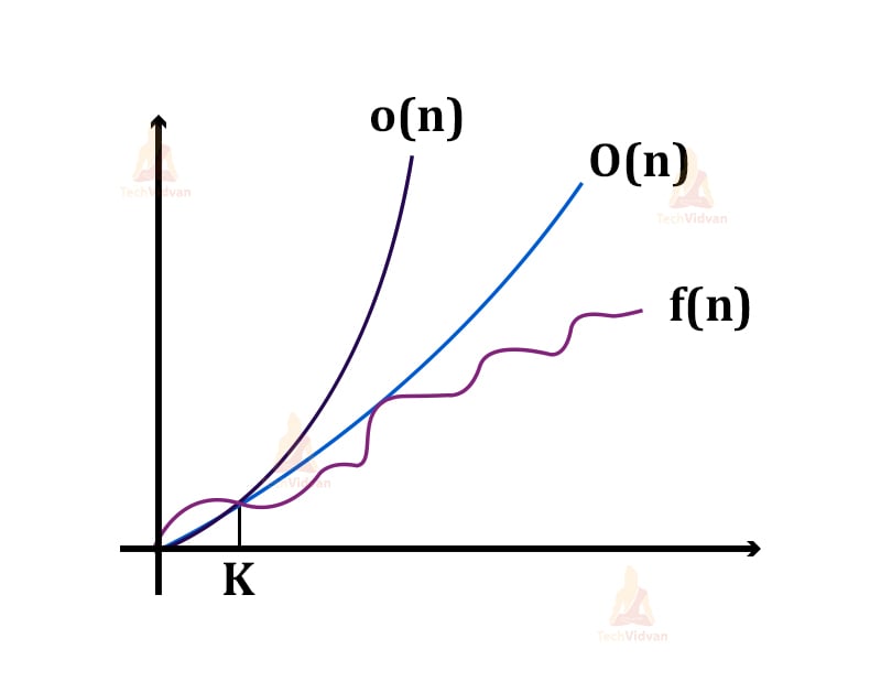
Then, f(n) will be o(g(n)) i.e. f(n) = o(g(n)) for a given constant ‘k’ such that k>1
If 0 ≤ f(n) ≤ c.g(n)
where, c = a constant and c>0
From here, we can say that after the point n=k in the graph, the function f(n) never grows faster than g(n). Thus, we are calculating the approximate growth of a function rather than the exact growth.
2. Little ω notation
a. Just like the omega notation(Ω), the little ω notation provides the lower bound for a function.
b. However, the Ω notation provides the tightest lower bound and the little-omega provides a loose lower bound for the function.
c. Just like little-o notation, ω gives the estimation of growth and not the actual growth for a function f(n).
For example, consider the graphs f(n) and g(n) as shown below:

Then, f(n) = ω(g(n)) if for a given constant ‘c’ such that c>0 and ‘k’ such that k>=1
f(n) > c.g(n) >=0.
Advantages of Asymptotic notations
1. Asymptotic notations help us represent the upper and lower bound of execution time in the form of mathematical equations.
2. It is not feasible to manually measure the performance of the algorithm as it changes with the input size. In such a case, asymptotic notations help us give a general insight into execution time for an algorithm.
3. Asymptotic analysis is so far the most efficient and the best way to analyse algorithms against the actual running time.
4. Asymptotic analysis helps us in performing our task with fewer efforts.
Common asymptotic notations
1. These are some most commonly used asymptotic analysis.
2. The table below shows them in the increasing order of their running time i.e. O(1) takes less execution time than O(log n) and so on.
| Constant | O(1) |
| Logarithmic | O(log n) |
| Linear | O(n) |
| n log n | O(n log n) |
| Quadratic | O(n2) |
| Cubic | O(n3) |
| Polynomial | nO(1) |
| Exponential | 2O(n) |
Here, I have given only worst-case complexities for common types of equations because we are mostly interested in how an algorithm will behave in the worst-case.
Time complexity of some most commonly used algorithms
Let us see the worst-case time complexities of some important searching and sorting algorithms:
1. Searching techniques:
| Algorithm | Worst-case complexity |
| Linear search | O(n) |
| Binary search | O(log n) |
2. Sorting techniques:
| Algorithm | Worst-case complexity |
| Insertion sort | O(n2) |
| Selection sort | O(n2) |
| Bubble sort | O(n2) |
| Merge sort | O(n logn) |
| Quicksort | O(n2) |
| Radix sort | O(nk) |
| Bucket sort | O(n2) |
Conclusion
Without asymptotic analysis, we can’t judge which algorithm is the most suitable for us.
Suppose we wish to calculate the sum of first n natural numbers. One algorithm does that in O(1) time and the other algorithm takes O(n) time in the worst-case. Having their asymptotic analysis, we surely know that the first algorithm will be faster and more efficient.
This is why the study of asymptotic analysis is the fundamental step to learn the working of algorithms.