Divide and Conquer Algorithm with Applications
1. As the name suggests, ‘Divide and Conquer is a strategy in which a given problem is split into a set of subproblems.
2. Each sub-problem is then handled/solved individually.
3. Once all the sub-problems are solved, we combine the sub-solutions of these subproblems and find the final solution.
Divide and Conquer
Divide and Conquer is broadly a 3-step strategy:
1. Divide the actual problem into sub-problems (A subproblem is just a smaller instance of the same problem).
2. Conquer i.e. recursively solve each sub-problem.
3. Combine the solutions of the sub-problems to get the solution to the actual problem.
For example, Let there be a problem of size N and let us divide this problem into 4 sub-problems say n1, n2, n3, and n4.
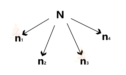
Let the time taken to complete the whole problem be T(N), time taken to complete n1, n2, n3, n4 respectively be T(n1), T(n2), T(n3) and T(n4), time taken in dividing the problem into sub-problems be D(N), time taken to combine the solutions of sub-problems into one final solution be C(N).
Then,
T(N) = T(n1) + T(n2) + T(n3) + T(n4) + D(N) + C(N) (If N is large)
T(N) = g(n) (If N is small)
Fundamentals of Divide and Conquer
The Divide and Conquer strategy follows two fundamentals:
1. Relational formula
a. It is the first thing required to solve a problem by divide and conquer effectively.
b. The relational formula is the formula that we generate for a given technique.
c. We need this formula to apply divide and conquer, break the problem into sub-problems and then solve them recursively.
2. Stopping condition
a. It defines the point at which we need to stop dividing our main problem into sub-problems and start combining the results that we get out of sub-problems.
b. We can also say that the stopping condition defines the base case of our recursive algorithm.
General algorithm for Divide and Conquer
Consider a problem named DAC having array ‘a’, smallest index as ‘i’ and the largest index being ‘j’.
DAC(a, i, j){
  if(small (i,j))
    return solution(small(i, j))
  else{
    m = Divide(i, j);
    b = DAC(a, i, m);
    c = DAC(a, m, j);
    d = Combine(b,c);
  }
}
Divide and Conquer recurrence relation
Divide and conquer is a recursion based algorithm. So, it will have a recurrence relation that mathematically defines its behaviour.
The recurrence relation for Divide and conquer is:
T(n) = aT(n/b) + f(n), where a > 1 and b > 1
Time complexity
Let us solve this recursive function using the Master’s equation. Master’s theorem is a simple and direct method to find a solution for recurrence relations:
We take into consideration the three following cases:
1. If f(n) = Θ(nc) then T(n) = Θ(nlogba) , here c < logba
2. If f(n) = Θ(nc) then T(n) = Θ(nclog n) , here c = logba
3. If f(n) = Θ(nc) then T(n) = Θ(f(n)) , here c > logba
For example,
1. Let T(n) = 4T(n/2) + n (log n). Here, a=4, b=2, k=1.
Therefore, Logba = log24 =2 and k=1, thus Logba > k
So, T(n) = Θ(n2)
2. Let a recurrence relation be : T(n) = 2T(n/2) + cn. Here a=2,b=2,k=1.
Then, Logba = log22 =1 = k.
So, T(n) : Θ(nlog2(n)).
In case of Merge sort
The recurrence relation will be: T(n) = 2T(n/2) + Θ(n). Here, c=1 and logba=1. Therefore, the complexity of merge sort is Θ(n log n).
Advantages of Divide and Conquer Algorithm
1. The divide and conquer algorithm solves all the problems recursively, so any problem, which requires recursion can make use of Divide and conquer.
2. The Tower of Hanoi was one of the biggest mathematical puzzles. But the divide and conquer algorithm has successfully been able to solve it recursively.
3. The divide and conquer divides the problem into sub-problems which can run parallelly at the same time. Thus, this algorithm works on parallelism. This property of divide and conquer is extensively used in the operating system.
4. The divide and conquer strategy makes use of cache memory because of the repeated use of variables in recursion.
5. Executing problems in the cache memory is faster than the main memory.
6. Brute force technique and divide and conquer techniques are similar but divide and conquer is more proficient than the brute force method.
7. The divide and conquer technique is quite faster than other algorithms.
Disadvantages of Divide and Conquer Algorithm
1. The divide and conquer technique uses recursion. Recursion in turn leads to lots of space complexity because it makes use of the stack.
2. The implementation of divide and conquer requires high memory management.
3. Memory overuse is possible by an explicit stack.
4. The system may crash in case the recursion is not performed properly.
Divide and conquer algorithm vs dynamic programming
1. Both divide and conquer make use of recursion for finding a solution to a problem, but both of them have different properties and thus a different problem set.
2. In both divide and conquer as well as dynamic programming, we divide the given problem into multiple sub-problems and then solve those sub-problems.
3. In dynamic programming, the same problem is required to be solved again and again.
4. However, in divide and conquer, we divide the problem into separate sub-problems and calculate all of them once. Then we combine their results.
For example, in the merge sort algorithm, we use the divide and conquer technique, so that there is no need to calculate the same subproblem again.
However, when we calculate the Fibonacci series, we need to calculate the sum of the past two numbers again and again to get the next number.
This is why solving the Fibonacci series requires dynamic programming.
Let us understand the comparison between dynamic programming and divide and conquer algorithm with the help of merge sort and Fibonacci series:
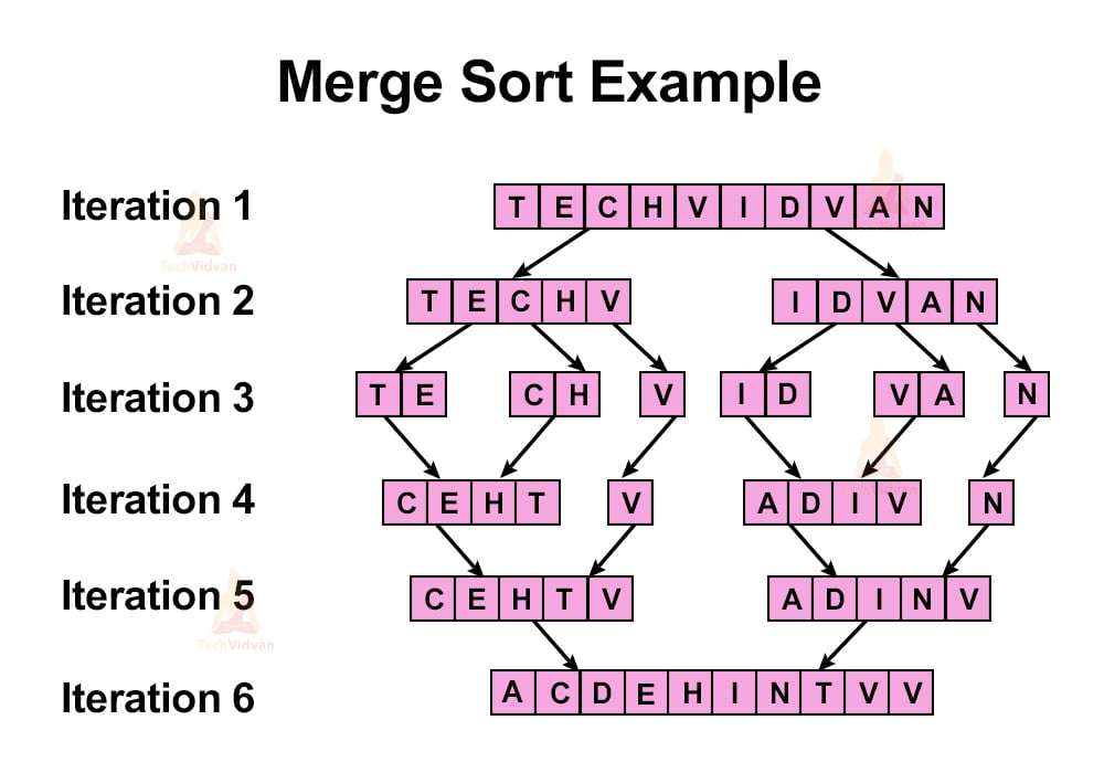
1. Merge sort:
Suppose we wish to arrange the letters of the word ‘TECHVIDVAV’ in ascending order. Then,
2. Fibonacci series:
Write an algorithm in dynamic programming that generates the Fibonacci series.
Member=[ ];
fibonacci(n){
    if  n in Member
        return member[n];
    else{
      if( n < 2)
 fib= 1;
      else
 fib = fib(n - 1) + fib(n -2);
    }
    mem[n] = fib;
    return fib;
}
Write a function that generates the Fibonacci series using the divide and conquer approach.
fibonacci(n){
    If n < 2
        return 1;
    else
        return fib(n - 1) + fib(n -2);
}
Applications of Divide and Conquer
Divide and conquer strategy has various application areas such as:
1. Defective chessboard
2. Binary search
3. Finding the maximum and minimum in an array
4. Merge sort
5. Quicksort
6. Strassen’s matrix multiplication
and many more.
Let us discuss a few of these applications in detail:
1. Min-Max analysis
Consider an array ‘a’ having 6 elements as shown:
| 5 | 16 | 1 | 2 | 3 | 18 |
Steps involved:
1. Since we don’t know the largest element, so let us consider the first element of ‘a’ to be the maximum element and store it in a variable named ‘max’.
2. Check whether a[i] > max or not. If not, return max itself directly.
3. If a[i] > max, then assign the value of a[i] to max and then return max.
This process continues for all the elements of the array until we find the maximum value.
2. Brute force method (Iterative approach)
The maximum or minimum value in an array can simply be found by comparing all the elements inside a loop as shown:
FindMax(A, n){
  int i;
  max = A[0];
  for(i=1; i<n; i++){
    If(A[i] > max)
      max = A[i];
  }
  Return max;
}
Here, we have simply met through with an iterative approach.
The total number of comparisons involved in this method is n-1, where n is the number of elements in the array.
The above was the method to find the maximum element of an array. Now if we wish to calculate the minimum element likewise, then total comparisons will be
Total comparisons = (n-1) + (n-1) = 2(n-1).
Divide and conquer approach:
In divide and conquer, we will divide the problem into smaller parts. Let us suppose we have divided the problem into 2 sub-parts.
Then sub-part1 will be the first half of the array whereas sub-part2 will be the second half of the array. Both the sub-parts will have their own set of ‘max’ and ‘min’ i.e. (max1, min1) and (max2, min2).
While combining the sub-solutions, we will see which of the max’s is larger in between max1 and max2 and that will be the final answer. Similar is the case of the min value.
Let A be an array with starting index ‘i’ and ending index ‘j’. Let ‘min’ denote the minimum value and ‘max’ denote the maximum value. Then,
DAC_min_max(A, i, j, min, max){
  if(i == j)
    min = max = a[i]; // i.e. an array of size 1 having only 1 element
  else if(i == j-1){
    if(a[i] < a[j]){
      min = a[i];
      max = a[j];
    }
    else{
      min =  a[j];
      max = a[i];
    }
  }
  else{
    m = (i+j)/2;
    min1, max1 = DAC_min_max(A, I, m, min, max);
    min2, max2 = DAC_min_max(A, m+1, j, min, max);
    if(min1 < min2)
      min = min1;
    else
      min = min2;
    if(max1 > max2)
      max = max1;
    else
      max = max2;
  }
  return min, max;
}
Here, we are returning 2 values- min and max, which never happens in the real case because a function can return only 1 value. But since this is a pseudo-code and just for the sake of explanation and simplicity, I have assumed that the function is returning both min and max.
Also, we have taken 2 separate cases here:
1. When n=1 i.e. when the array has only one element.
2. When n=2 i.e. when the array has 2 elements. Now we have taken a separate case for n=2 because 2 is a small number and it could be performed directly. If we would have applied DAC, then also, it would have worked, but that would have been an unnecessary load on the program. This is because divide and conquer makes use of recursion for implementation. Recursion requires stack i.e. unnecessarily increasing the complexity of the program. This could be avoided by taking a separate case for array size 2.
3. When n is any positive value other than 1 and 2.
Here,
T(n) = T(n/2) + T(n/2) + 2, n>=2
‘2’ is for two comparisons in the algorithm (one comparison for ‘min’ and another for ‘max’).
3. Binary search
Binary search is also implemented by the divide and conquer strategy. This is used to find a particular element in a sorted array.
While implementing binary search, we divide the array into 2 halves and check if the number to be searched could be on the left half or right half. Then, we go to that half and again divide the array into further two halves. This process goes on until the number to be searched is found.
Note:- There is another thought of school which says that binary search does not come directly under the divide and conquer. Rather, it is implemented using an altogether different methodology named ‘Decrease and Conquer’.
Let us see the implementation of binary search using an example:
Given a sorted array ‘A’ of size ‘n’ we need to find the position of an element, say ‘x’ in A. let i be the starting index and j be the last index.
Let A contain the following elements:
| 10 | 20 | 30 | 40 | 50 | 60 | 70 | 80 |
The first step is to find the mid of the array.
Here, the middle element would be (0+7)/2 = 3
The algorithm for binary search will be as follows:
BSearch(A, i, j, x){
  if(i == j){
    if(A[i] == x)
      return I;
    else
      return -1;
  }
  mid = (i + j)/2;
if(A[mid] == x)
    return mid;
  else if(x < A[mid])
    return BSearch(A, i, mid-i, x)
  else
    return Bsearch(A, mid+1, j, x)
}
The time complexity of the binary search algorithm is O(log n). Here, a log to base 2 is considered.
Thus, we can say that a binary search is better than a simple linear search algorithm. This is because a linear search has a time complexity of O(n) which is much higher than a binary search’s complexity.
4. Bubble sort
a. In bubble sort, we compare each pair of elements, and if they are not in order, then swap them.
b. This sorting technique is very time-consuming has a high complexity of O(n2). Thus, it is not suitable for large input sizes.
c. While sorting a list using a bubble sort, the last element will settle first at its final position.
d. This is why the modified algorithm does not perform the last iteration in the loop after each iteration.
5. Quicksort
a. This is one of the most efficient sorting algorithms.
b. It selects a pivot value from an array and then divides the rest of the array elements into two subarrays one on the right side of the pivot and the other on the left side.
c. It then compares the pivot element to each element and sorts the array recursively.
d. The algorithm for quicksort is shown below:
Algorithm QuickSort(p,q){
    //Sort the elemnets a[p]....a[q] which reside in the
    //global array a[1:n] into ascending order;
    if(p<q){   //If there are more than 1 elemnets
        //Divide p into sub-problems
        j := partitionArray(a, p, q+1);
            //j is the position of the partitioning element.
        //Solve the sub-problems.
        QuickSort(p, j-1);
        QuickSort(j+1, q);
    }
}
6. Merge sort
a. It divides the given array into halves which further divide themselves into two halves until the array length becomes one.
b. It then starts merging the two sorted halves from bottom to top until we get the final sorted array.
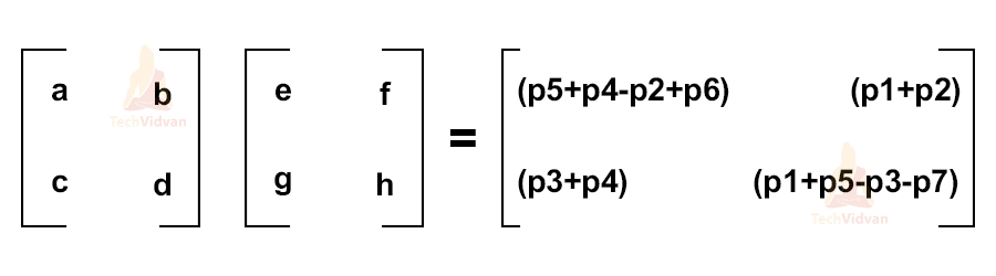
7. Strassen’s algorithm
a. This algorithm is used for matrix multiplication using the divide and conquers strategy.
b. When the input size is large, this algorithm proves to be much faster than the brute force techniques for performing matrix multiplication.
c. The algorithm divides the matrix of order N into two separate matrices each of order N/2.
d. It performs the multiplication for sub-matrices using the following results:
p1 = a(f-h) p2 = (a + b)h
p3 = (c + d)e p4 = d(g- e)
p5 = (a + d)(e+ h) p6 = (b-d)(g+h)
p7 = (a-c)(e+f)
8. Closest pair of points
a. Given N points in matrix space, this algorithm is used to find the points that are closest to each other in the space.
b. It is a problem of computational geometry.
9. Karatsuba algorithm for fast multiplication
a. It is one of the fastest algorithms for the multiplication of two numbers.
b. Let us understand this algorithm with the help of an example:
Let there be two numbers: X and Y.
Step 1: Divide the numbers into two halves as shown:
X = Xl*2n/2 + Xr
Y = Yl*2n/2 + Yr
Here,
Xl, Yl: contains leftmost N/2 bits of numbers X and Y respectively.
Xr, Yr: contains rightmost N/2 bits of numbers X and Y respectively.
Step 2: Perform their multiplication i.e. X*Y
XY = 2n XlYl + 2n/2 * [(Xl + Xr)(Yl + Yr) – XlYl – XrYr] + XrYr
The complexity of the Karatsuba algorithm is O(n1.59) which is better than the brute force approach which had the time complexity of O(n2).
Conclusion
This article gives details of what a divide and conquer approach looks like and some real-life applications of this strategy. This article also gives insights into how to solve the divide and conquer problems recursively.
Thus, divide and conquer is one of the most important strategies in algorithm design and has multiple real-life applications.