Greedy Algorithm with Applications
We encounter various types of computational problems each of which requires a different technique for solving. A problem that requires a maximum or minimum result is the optimization problem.
There are broadly 3 ways to solve optimization problems:
1. The greedy method
2. Dynamic programming
3. Branch and bound technique
This article will cover the greedy method, properties of greedy algorithms and the steps to implement the greedy method over any problem.
What is Greedy Algorithm?
It simply means to pick up a choice/solution that seems the best at the moment ( being greedy). This technique is best suited when we want an immediate situation. It helps to solve optimization problems i.e. which gives either minimum results or maximum results.
A solution satisfying the condition in the problem is a feasible solution. The solution having minimum cost out of all possible feasible solutions is the optimal solution i.e. it is the best solution.
The goal of the greedy algorithm is to find the optimal solution. There can be only 1 optimal solution.
For Example:
Let us consider the example of the container loading problem.
In a container loading problem, a large ship is loaded with cargo. The cargo has containers of equal sizes but different weights. The cargo capacity is of the ship is cp.
We need to load the containers in the ship in such a way that the ship has maximum containers.
For example, let us say there are a total of 4 containers with weights: w1=20, w2=60, w33=40, w4=25.
Let cp = 80. Then, to load maximum containers we will load container-1,3,4.
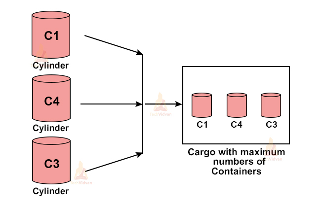
We will load the containers in the order of increasing weights so that maximum containers load inside the ship. Here, the order of loading is container1→container4→container3.
History of Greedy Algorithm
The greedy algorithm was first coined by the Dutch computer scientist and mathematician Edsger W. Dijkstra when he wanted to calculate the minimum spanning tree. The major purpose of many greedy algorithms was to solve graph-based problems.
The greedy algorithms first started coming into the picture in the 1950s. The then scientists, Prim and Kruskal also achieved the optimization techniques for minimizing the costs of graphs during that decade.
A few years later, in the 1970s, many American researchers proposed a recursive strategy for solving greedy problems. In 2005, the NIST records registered the greedy paradigm as a separate optimization strategy.
Since then, the greedy algorithm has been extensively in use in multiple fields including the web protocols such as the open-shortest-path-first (OSPF) and many other network packet switching protocols.
Working of Greedy Algorithm
The greedy algorithm works in various stages and considers one input at a time while proceeding. At each stage, we try to find a feasible solution for our problem, a solution that is good for the algorithm at that point. This means that we make a locally optimal choice for each sub-task. These local optimal choices eventually lead us to the global optimal choice for our problem which we call the final optimal solution.
The pseudo-code for the simplest greedy algorithm is shown below:
ALgorithm Greedy(A,n)
{
    solution := ϕ; //Initializing the solution
    for i:= 1 to n do
    {
        x := select(A);
        if Feasible(solution,x) then
            solution := Union(solution, x);
    }
    return solution;
}
Here, A = an array of size n.
The select function takes an input from the array and removes it. We assign this selected input value to x.
Feasible is the boolean function that decides whether we can include x in the final solution vector or not. A good greedy algorithm has a proper implementation of select, Feasible and Union.
Properties required for the Greedy Algorithm
There are many techniques to solve a problem. Out of these many techniques, we have optimization techniques for a particular set of problems. Out of optimization techniques as well, there are multiple choices.
So, how do we know that when to use and when not to use the greedy method as an optimization algorithm.
For this purpose, we will check the properties of the algorithm. If the following two properties hold, we will use the greedy approach or other approaches.
1. Greedy choice property
To reach the final optimal solution or the globally optimal solution, we find locally optimal solutions(the best at that moment) for each sub-task.
2. Optimal sub-programs
A solution to the subproblem of an optimal solution is also always optimal.
Characteristic of a Greedy Approach
1. In the greedy method, we divide the main problem into sub-problems and solve each of them recursively.
2. The greedy method maximizes the resources in a given time constraint.
3. There is a cost and value attribution attached to these resources.
Steps to achieve Greedy Algorithm
1. Feasible
The greedy algorithm proceeds by making feasible choices at each step of the whole process. Feasible choices are those which satisfy all the algorithmic constraints.
2. Local optimal choice
Choose what is best at the given time i.e. make locally optimal choices while preceding through the algorithm.
3. Unalterable
We cannot alter any sub-solution at any subsequent point of the algorithm while execution.
When to use Greedy Algorithm?
Greedy algorithms always choose the best possible solution at the current time. This sometimes leads to overall bad choices and might give worst-case results.
For example, Suppose we wish to reach a particular destination and there are different paths for it, as shown below:
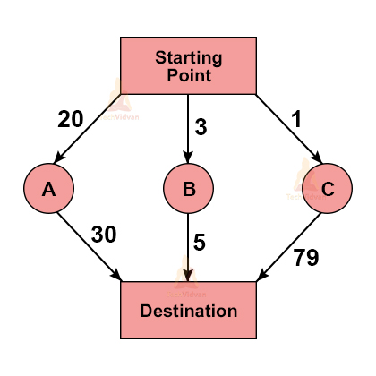
Here, following path ‘A’ will cost us 50, path ‘B’ will cost 8(minimum) and path ‘C’ will cost us 80.
If we follow the greedy approach, we will first move from starting point to node ‘C’ because it has the minimum cost at that point. But in reality, this path has the maximum total cost. However, we were not able to detect it at the first step.
Following the greedy method will cost us the maximum here i.e. 80. In such cases, the greedy approach might not give optimal results.
So the question arises- When to use the greedy approach.
We use this technique because it gives optimal results in many cases by just making ‘layman moves’. We also prefer greedy methods whenever we are sure that they will provide us with good approximations. In such cases, the greedy approach proves to be very effective as it is cheaper and faster.
Advantages of Greedy Algorithm
1. It is a highly optimized and one of the most straightforward algorithms.
2. This algorithm takes lesser time as compared to others because the best solution is immediately reachable.
3. In the greedy method, multiple activities can execute in a given time frame.
4. We don’t need to combine the solutions of sub-problems, as it automatically reaches the optimal solution.
5. The algorithm is easy to implement.
Applications of Greedy Method
There are multiple applications of the greedy technique such as:
1. CPU Scheduling algorithms
CPU scheduling is a process that allows and schedules more than one processes in a CPU at a time so that there is maximum utilization of the CPU.
This usually happens when one process is on hold due to the unavailability of resources, and to avoid CPU time wastage, we schedule a new process for the time.
Multiple algorithms help in CPU scheduling and they make use of the greedy approach. The purpose of these algorithms is to maximize CPU utilization and minimize the time taken by a process to execute.
There are various types of scheduling algorithms:
a. First come first serve
As the name suggests, it schedules processes based on first come first serve. It is a non-preemptive algorithm.
b. Shortest job first
It is both preemptive as well as non-preemptive scheduling algorithm. In this algorithm, we give the highest priority to process with the lowest burst time. Its preemptive version is known as the Shortest job first algorithm.
c. Priority scheduling
It is both preemptive or non-preemptive. In this technique, we assign priority to every process and then execute in the priority order. It mostly uses a priority queue for execution.
d. Round-robin scheduling
In this algorithm, we assign a fixed time slot to each process. If the process does not execute completely in that time slot, it will complete its remaining execution in the next rounds. It is preemptive.
e. Multiple level queue schedule
This is also a priority-based algorithm. It maintains multiple queues for the processes with different priorities.
2. Minimum spanning trees
A minimum spanning tree is a subset of a connected, weighted undirected graph that connects all the vertices without cycle. In MST, the total weight of all the edges is minimum.
3. Dijkstra shortest path algorithm
This algorithm is used to find the shortest path between two vertices in a graph in such a way that the sum of weights between the edges is minimum. All those algorithms in which we need to maximize or minimize something make use of the greedy approach.
4. Fit algorithm in memory management
This algorithm allocates different memory blocks to the processes in an operating system.
In the fit algorithm, we make use of a pointer to keep track of all memory blocks available to us. The pointer also decides whether to accept or reject the request for memory block allocation for any incoming process. It makes this decision depending on three different fit memory management algorithms:
a. First fit algorithm
The pointer allocates that memory block to the process which it first finds to be sufficient for the process.
b. Best fit algorithm
The algorithm allocates the minimum sufficiently available memory block to the process.
c. Worst fit algorithm
It allocates the largest sufficient memory block available in the memory.
5. Travelling salesman problem
This is one of the standard problems that a greedy algorithm solves. In this problem, our objective is to make use of the greedy technique to find the shortest possible path. The objective is to visit each city exactly once and then return to the initial starting point.
6. Fractional knapsack problem
It is an optimization problem. In the fractional knapsack problem, we try to find a subset of items out of the total possible set of items. We ensure that their total weight is less than or equal to a given limit according to the problem. We also ensure that their value is maximum.
7. Egyptian fraction
It is a finite sum of unique distinct fractions. We can represent every positive fraction as a sum of unique unit fractions which we call the Egyptian fraction.
8. Bin packing problem
In the bin packing problem, we have a finite number of bins of fixed volume. We pack items of different volumes into those bins in such a way that we use the minimum number of bins.
Limitations of Greedy Algorithm
The greedy method works by finding the best possible outcome at every step of the algorithm. This sometimes leads to inaccurate results.
For example, suppose we wish to find the longest path in the following graph:
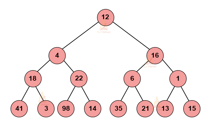
If we follow the greedy approach, we will make the best possible choice at every node. In that case, the path will come out to be: 12→16→6→35 which comes out to be 69.
However, in reality, the actual longest path is 12→4→22→98 which comes out to be 136. Here, achieving 136 is impossible using the greedy approach. In this case, the greedy algorithm gave the wrong results.
Problems solved by Greedy Method
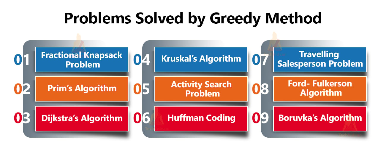
The greedy method is well versed to solve multiple types of problems. Some of them are:
1. Fractional knapsack problem
2. Prim’s algorithm
3. Dijkstra’s algorithm
4. Kruskal’s algorithm
5. Activity search problem
6. Huffman coding
7. Travelling salesperson problem
8. Ford- Fulkerson algorithm
9. Boruvka’s algorithm
Let us discuss all of these in detail.
1. Fractional Knapsack Problem
It is an optimization problem in which we can select fractional items rather than binary choices. The objective is to obtain a filling knapsack that maximizes the total profit earned.
Step 1: Calculate the ratio of value overweight for every item. If the weight is in pounds, calculate the value per pound.
Step 2: Sort the items depending on the ratio calculated in step 1.
Step 3: Take the item with the highest ratio i.e. take the maximum possible value of substance with the maximum value per pound.
Step 4: Suppose that the amount that we took in step 3 exhausts but we still have space. Then, we will take the further possible amount of substance with the further maximum value of weight.
i.e. we will take the next highest ratio.
Algorithm:
fractional_knapsack (array w, array v, int C)
{
    for i= 1 to size (v) do
        for i= 1 to size (v);
    sort_descending (vpp);
     i := 1;
     while (C>0) do{
         amt = min (C, w [i]);
         sol [i] = amt;
         C= C - amt;
          i := i+1;
     }
     return sol;
}
2. Prims algorithm
It is a greedy algorithm to obtain a minimum spanning tree. Its time complexity is of the order O(n2).
This algorithm builds the tree edge by edge, where it chooses the edge based on some optimization criterion. One of the criteria is to choose an edge in such a way that the increase in the sum of costs of edges is minimum.
The algorithm takes the input in the form of a graph. It then chooses the subset of edges of the graph in such a way that
a. The graph forms a tree including every vertex
b. The graph has the minimum sum of weight among all the subtrees.
Algorithm :
The steps are as follows:
1: Initialize a vertex for the minimum spanning tree.
2: Search for all the edges that connect the tree to new vertices.
3: Find the minimum of all those selected edges.
4: Add this value to the tree.
5: We will perform the above steps recursively to reach the minimum spanning tree.
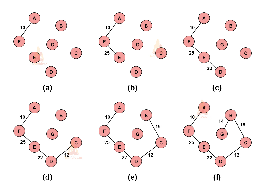
Stages in Prim’s algorithm:
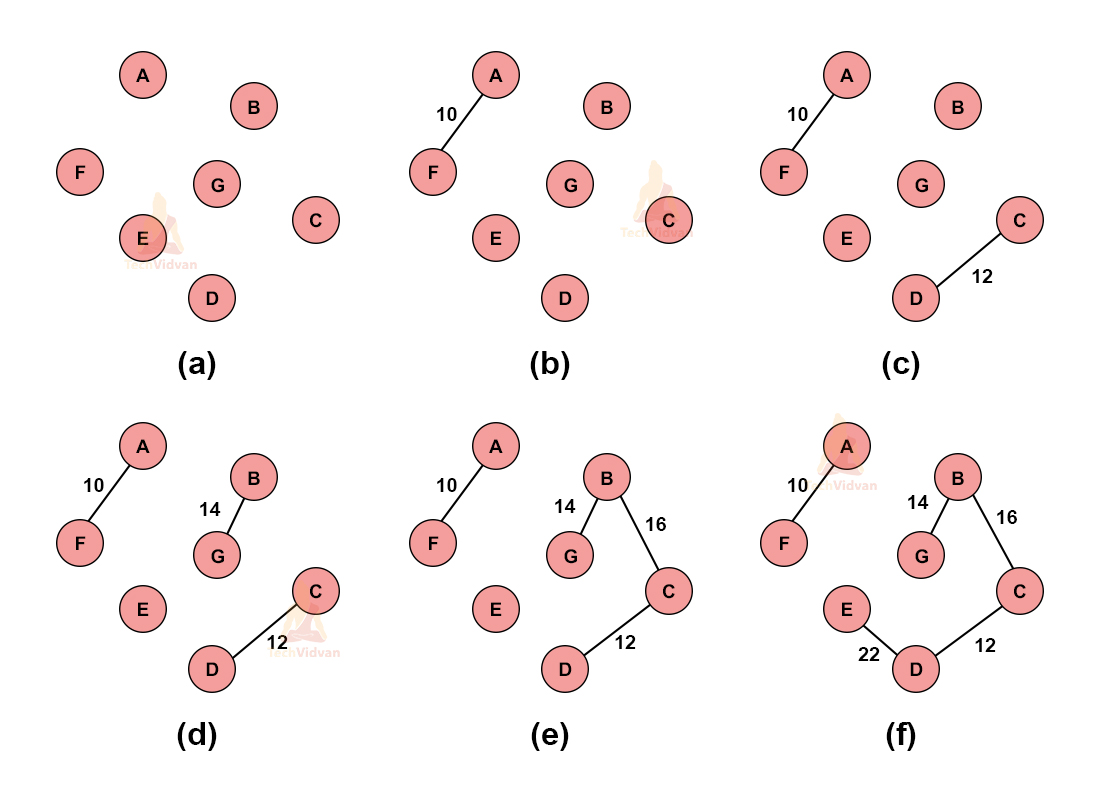
Let us look through an example to understand the stages in Prim’s algorithm:
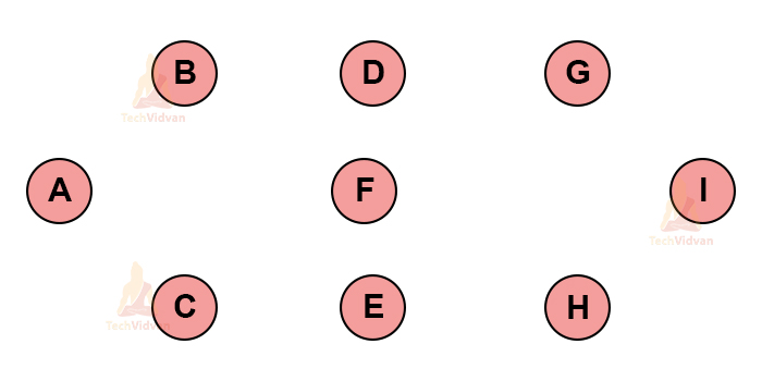
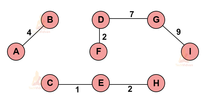
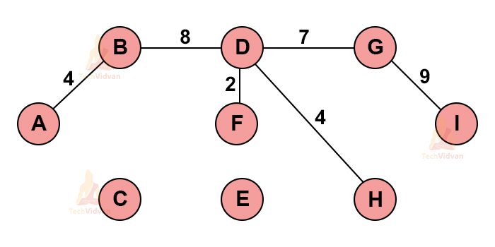
Consider the following graph.

1. Select any random vertex, say ‘A’ here.
2. Select the edge with the minimum weight from this node and add it to the existing node.
3. Choose the nearest vertex that we can include.
4. Repeat these above steps recursively to obtain based on the minimum spanning tree.
The various stages of spanning tree will be:
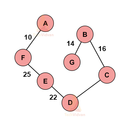
The final obtained spanning tree is:
3. Dijkstra’s algorithm
In a graph, there can exist multiple paths between a pair of vertices. But, if we wish o find the shortest possible path between any two vertices, we make use of Dijkstra’s algorithm. It may or may not include all the vertices.
It is somewhat similar to Prim’s algorithm and is used to find the shortest path just like Pri’s algorithm.
While executing, it maintains two different sets. One set contains those vertices which we have included in the shortest path. The other set contains the remaining vertices, which we haven’t included yet.
For example:
1. Consider the following graph:
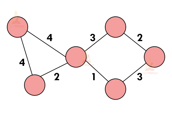
2. Select any vertex randomly. Consider it as the starting vertex.
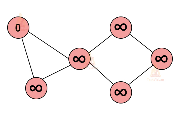
Consider the remaining vertices to be at an infinite distance from the starting vertex.
3. From the starting vertex, traverse to every immediate vertex. As we reach the particular vertex, we update its path in our graph.
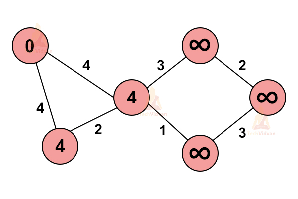
If the adjacent path of a particular vertex is greater than the current path, do not update the values.
4. Repeat step 3.
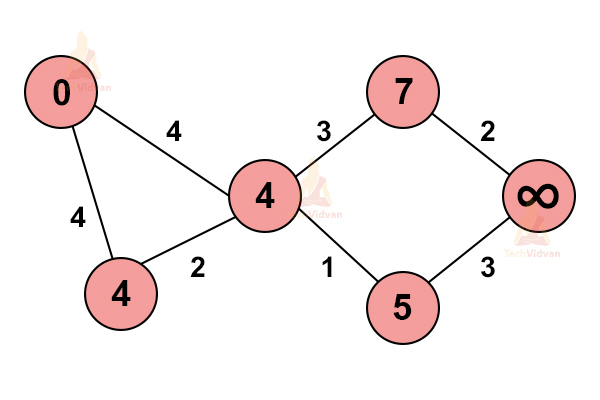
Do not change or update the path of those nodes which we have already visited once.
5. Check if there is still any unvisited node in the graph or not. If an unvisited node still exists, select the path with the shortest possible distance to reach that node.
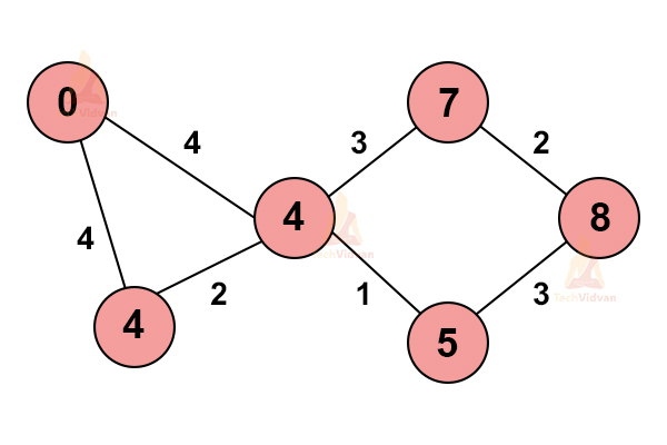
This is how we calculate the shortest path using Dijkstra’s algorithm.
4. Kruskal algorithm
It is another possible interpretation to find out the minimum spanning tree in a graph. A minimum spanning tree always has one edge less than the number of edges in the graph.
This algorithm also ensures that there are no loops created on adding edges to the tree.
Algorithm:
1. Sort all the edges of the graph in non-descending order of their weights.
2. Take the smallest edge.
3. Check whether it is forming a cycle or not with the spanning-tree formed so far.
4. If a cycle is found, discard this particular edge leading to the cycle. If there is no cycle, include the edge in the spanning tree.
5. Repeat the above steps until we have included all the vertices.
Example:
Consider the following graph:
a. We need to find the minimum spanning tree for this graph using Kruskal’s algorithm.
b. Select the edge having minimum weight. If multiple edges are having minimum weight, choose any one of them randomly.
c. Select the next shortest edge with the next minimum weight. Add it to the spanning tree.
d. Select the subsequent edges, in the same manner, depending on their weights.
e. Make sure that none of the added edges forms a cycle.
f. Repeat the above steps until we get our desired spanning tree.
Thus, the various stages of Kruskal’s algorithm are as follows:
5. Activity search problem
It is an optimization problem. This algorithm selects non-conflicting activities which we can perform in the given time frame. This problem schedules activities in the given intervals in such a way that maximum activities can be performed in the given time constraint.
Example:
1. Let there be ‘n’ activities ranging from 1 to n in a given set i.e. let S = {1,2,3,4,5,………,n-1, n}.
2. Only one activity can use a resource at a time i.e. the resources are non-sharable.
3. Let the start time for these ‘n’ activities be s1, s2, s3, s4,……sn.
4. Let the finish time of these activities be f1, f2, f3,f4,……….fn.
5. Consider two random activities ‘i’ and ‘j’. Then, let the interval of activity ‘i’ be [si, fi) and the interval of activity ‘j’ be (sj, fj).
In this case, activities ‘i’ and ‘j’ will be compatible only when their intervals i.e. [si, fi) and (sj, fj) respectively, do not overlap.
Activity search problem Algorithm:
Algorithm Activity_Selector(s, f)
{
    n := len[s];
    A := {1};
    j := 1;
    for i := 2 to n do{
        if (si ≥ fi) then
            A := A U {i};
        j := i;
    }
    return A;
}
Let us consider an example to understand the activity/task scheduling problem.
Suppose there are 7 tasks named a,b,c,d,e,f,g.
The following table gives the starting and finishing time for each task:
| TASK | START TIME | FINISH TIME |
| a | 0 | 2 |
| b | 3 | 7 |
| c | 4 | 7 |
| d | 9 | 11 |
| e | 7 | 10 |
| f | 1 | 5 |
| g | 6 | 8 |
Our objective is to assign these tasks to the computer in such a way that no two tasks overlap. We can make use of multiple machines. But since this is a greedy approach, we need to minimize the number of machines that we use for performing these tasks.
Initially, we will consider that the number of machines used = number of tasks i.e. we are assigning each task to an individual machine. In this case, the number of machines = 7(M1, M2, M3, M4, M5, M6, M7).
We will try to optimize the problem by minimizing the number of machines and at the same time, prevent overlapping. Thus, the final optimized schedule will be:
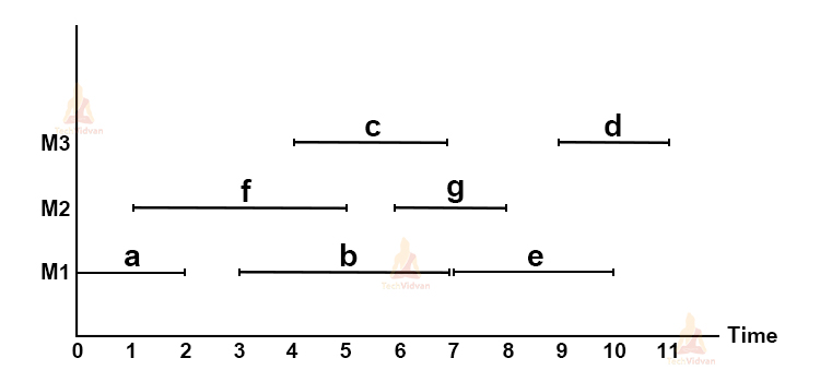
Here, we can clearly see that we were able to schedule all the activities in three turns or by using three machines i.e. M1, M2 and M3.
6. Huffman Coding
Huffman coding algorithm is used to compress data without the loss of any information from it. Each code is a binary string used for transmitting corresponding messages. A decode tree decodes at the receiving end.
Huffman coding assigns codes in such a way that the most frequent character gets the lowest code and vice versa. For this purpose, the algorithm maintains a table depicting the occurrence/frequency of characters.
| Character | a | e | i | o | u |
| frequency | 45 | 13 | 12 | 14 | 16 |
This table shows that ‘a’ occurs 45 times in the string, ‘e’ occurs 13 times and so on.
Here, a occurs maximum number of times, therefore it will have the lowest code.
Total bits required:= ( 45*1+13*4+12*4+14*3+16*3 )*1000 = 210,000 bits.
| Character | code |
| a | 0 |
| e | 101 |
| i | 110 |
| o | 100 |
| u | 111 |
Fixed length Code:
It assigns 3 bits to each character. Thus, for the whole file, we will need 3 x 106 bits.
Variable-length code:
It assigns long bits to less frequent characters and short bits to more frequent characters.
Huffman Coding Algorithm:
Huffman_codes(C)
{
    n=|C|;
    Q := C;
    for i=1 to n-1 do{
        z= allocate-Node ();
        x = left[z]=Extract-Min(Q);
        y= right[z] =Extract-Min(Q);
        arr [z]=arr[x]+arr[y];
        Insert (Q, z);
    }
    return Extract-Min (Q);
}
7. Travelling Salesman Problem
This problem states that there is a salesman who needs to visit a given set of cities starting from a particular city. We need to design the algorithm in such a way that the salesman cannot visit a city more than once. Also, he needs to return to the starting point after visiting all the cities.
We need to find the minimum possible path for the salesman to travel across all the cities. We make use of an adjacency matrix to depict the connected cities.
Consider a set of N cities- C1, C2, C3……Cn. let the cost of travelling be Tij for travelling between Ci and Cj.
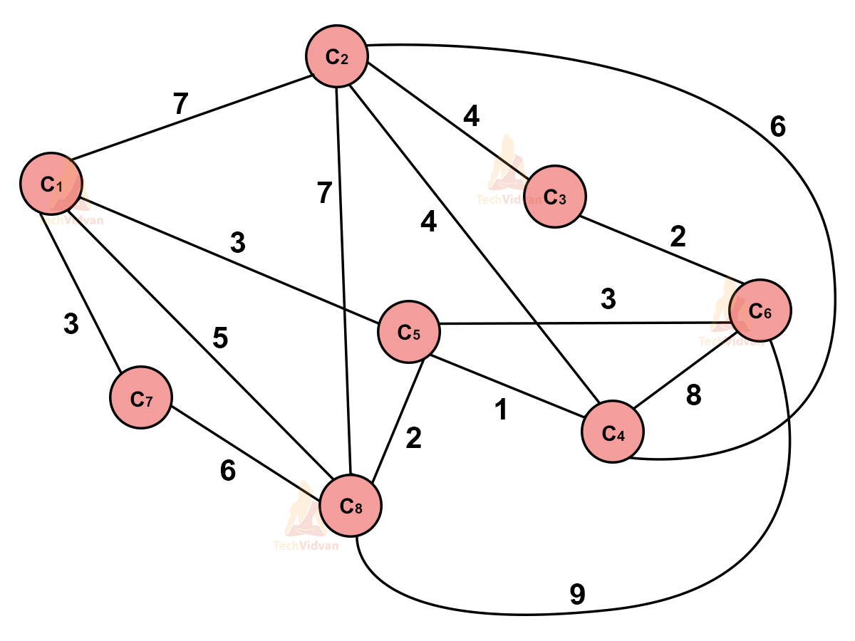
The adjacency matrix for the above path will be as follows:
| C1 | C2 | C3 | C4 | C5 | C6 | C7 | C8 | |
| C1 | 0 | 7 | 0 | 0 | 3 | 0 | 3 | 5 |
| C2 | 7 | 0 | 4 | 6 | 0 | 0 | 0 | 7 |
| C3 | 0 | 4 | 0 | 0 | 0 | 6 | 0 | 0 |
| C4 | 0 | 6 | 0 | 0 | 1 | 8 | 0 | 0 |
| C5 | 3 | 0 | 0 | 1 | 0 | 3 | 0 | 2 |
| C6 | 0 | 0 | 6 | 8 | 3 | 0 | 0 | 9 |
| C7 | 3 | 0 | 0 | 0 | 0 | 0 | 0 | 6 |
| C8 | 5 | 7 | 0 | 0 | 2 | 9 | 6 | 0 |
Thus, the shortest path is: C1→C5→C4→C2→ C3 →C6→C8→C7→C1
Cost = 3 + 1 + 6 + 4 + 6 + 9 + 6 + 3 = 38.
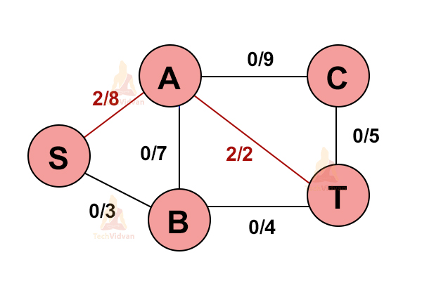
8. Ford – Fulkerson algorithm
This algorithm calculates the maximum possible flow in a graph. A flow network comprises vertices and edges with a source(S) and a sink (T).
All the vertices can both send and receive data equally. However, the source can only send the data whereas the sink can only receive the data.
Augmenting path: It is a path available in the flow network.
Residual graph: It is a flow network with the additional possible flow.
Residual capacity: It determines the capacity of an edge after removing the flow from maximum capacity.
Algorithm:
1. Initialize all the flow in the edges to zero.
2. If there exists an augmenting path between the source(S) and sink(T), add that path to the flow.
3. Update residual graph alongside.
Example:
Consider the following system of pipes with a fixed maximum capacity.

1. Select any path from S to T i.e. source to sink.
Let us select S→A→T.
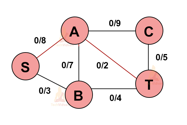
2. Update all the capacities in the graph.
Here, the minimum capacity is off the edge A → T(2).
3. Select another path S→B→A→C→T.
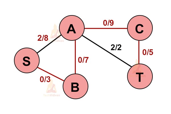
4. Update the capacities again.
Now the minimum capacity is from the edge S → B(3).
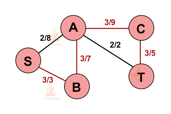
On adding all the flows i.e. 2+3, we get 5. Thus, this is the maximum flow possible.
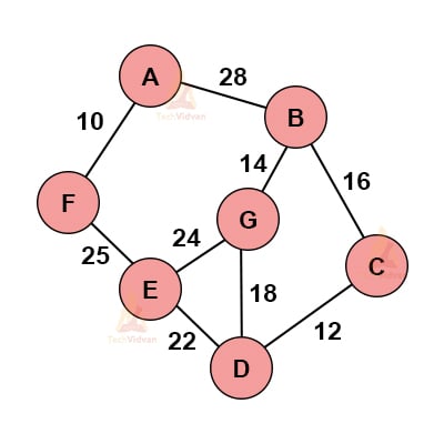
9. Boruvka’s algorithm
This algorithm is used to find the minimum spanning tree or forest in a graph. Using this algorithm, we can calculate the minimum spanning tree for a connected, weighted and non-directed graph.
For example, suppose we wish to calculate the minimum spanning tree for the following graph using Boruvka’s algorithm.
Step 1: The very first step is to initialize all the vertices as separate components as shown:
Step 2: Start from any vertex. Find the closest and the least weighted vertex and connect to the initial/starting vertex.
For example, let’s start from ‘A’. the closest components from ‘A’ are ‘B’ and ‘C’. Out of B and C, B has lesser weight. Therefore, we will draw an edge between A and B.
Step 3: Continue this process until all the nodes are traversed. The graph will look something like this.
Continue the process until we get the MST. Thus, the final MST is:
Greedy method vs Dynamic programming
| Greedy | Dynamic |
| In greedy, we select the current best and then try to solve the problem arising after it. | In dynamic, we select at each step, but it depends on the solution of subproblems. |
| This is more efficient at finding an optimal solution. | This is less efficient at finding an optimal solution. |
| It may or may not get an optimal solution, but it will always get a feasible solution. | This is less efficient but it guarantees the optimal solution |
| Example: fractional knapsack | Example: 0/1 knapsack |
Conclusion
The greedy method is one of the most important techniques for designing algorithms. This is primarily because it has many real-world applications and it applies to a wide variety of problems.
This article has given a fair idea of how to approach a problem using the greedy method. It also tells how and where we can use the greedy method and all the possible use cases of the algorithm.