Hash Table| Hashing in Data Structure
A Hash table is a type of data structure that makes use of the hash function to map values to the key. This data structure stores values in an associative manner i.e. it associates a key to each value. Hash tables make use of array data structures for storing values. The process or technique of mapping keys to the values is known as Hashing. The purpose of using hash tables as a data structure is to enable faster access.
What is a Hash Function?
A hash function is a function that maps keys to one of the values in the hash table. Hash functions return the location/address where we can store the particular key. We input the key to the hash function and the output is an address. The following diagram depicts the way a hash function operates:
For example, A possible hash function could be
h(k) = k mod m
Where h(k) denotes the hash function, m denotes the hash table size and k denotes the keys or values.
Characteristics of an Ideal Hash Function:
An ideal hash function has the following properties:
- Easy to compute
- For distinct keys, there must be distinct outputs.
- Uniformly distributed keys
Ways to Calculate Hash Functions:
There are three ways through which we can calculate hash functions:
1. Division method
2. Folding method
3. Mid square method
What is Hashing?
Hashing is a technique in which we make use of hash functions to search or calculate the address at which the value is present in the memory. The benefit of using this technique is that it has a time complexity of O(1). We calculate this address and store it in the hash table. We need to take care that the concept of hashing is applicable on distinct keys.
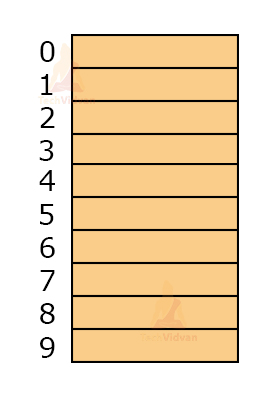
For example, let the hash function be h(k) = k mod 10 where k represents the keys. Let the keys be: 12, 11, 14, 17, 16, 15, 18 and 13. The empty table will look as follows having a table size of 10 and index starting from 0.
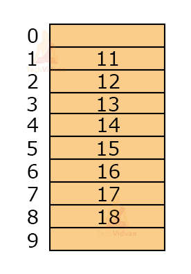
To insert values into the hash table, we make use of the hash function. h(12) = 12mod10 = 2
h(11) = 11mod10 = 1
h(14) = 14mod10 = 4
h(17) = 17mod10 = 7
h(16) = 16mod10 = 6
h(15) = 15mod10 = 5
h(18) = 18mod10 = 8
h(13) = 13mod10 = 3
The output of h(k) is the index at which we need to place the particular value in the hash table. Thus, after inserting values, the hash table will be:
Basic Operations on hash function:
The basic operations that we can perform on a hash function are:
1. Search: This operation helps to search an element from a hash table.
2. Insert: Insert operation is used to insert values into the hash table.
3. Delete: It is used to delete values from the hash table.
Collision in Hashing:
Collision is said to occur when two keys generate the same value. Whenever there is more than one key that point/map to the same slot in the hash table, the phenomenon is called a collision. Thus, it becomes very important to choose a good hash function so that the hash function does not generate the same index for multiple keys in the hash table.
For example, let keys be 10, 12, 23, 42, 51 and let the hash function be h(k) = k mod 10.
Then, h(12) = 12mod10 = 2
And, h(42) = 42mod10 = 2
Thus, both the keys 12 and 42 are generating the same index. So which value will we store in that particular index as we can store only one of them? This problem is solved by collision resolution techniques.
Collision Resolution Techniques:
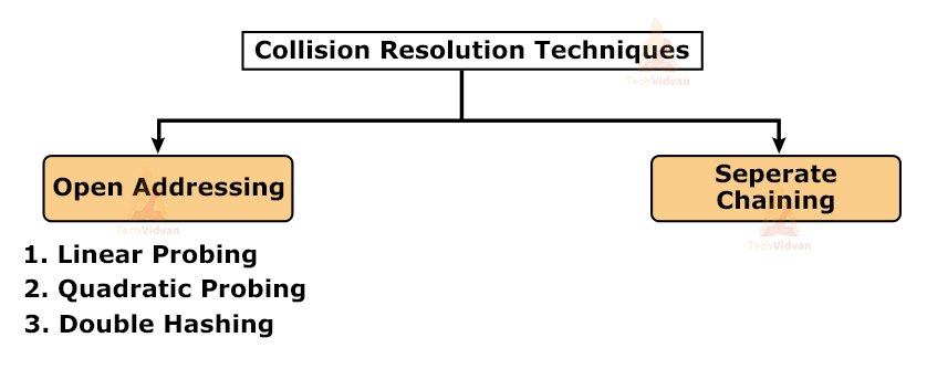
Collision resolution techniques come into use when a collision has occurred and we need to fix it. Broadly speaking, collision resolution techniques are divided into two categories:
1. Open addressing
2. Separate chaining
Open addressing also has various further categories used to resolve collision problems.
Open Addressing:
It is one of the collision resolution techniques. In this technique, we store all the keys in the table itself. Therefore, the size of the table has to be greater than or equal to the total number of keys present in the hash function. Open addressing comprises three different categories: Linear probing, quadratic probing and double hashing.
1. Linear Probing:
In linear probing, we look for the next empty slot linearly if the allotted slot is filled already. Let H denote the new hash function that will form after linear probing. Then,
H(k, i) = [ h(k) + i] mod m
Here, i is the collision number of the key where i = 0, 1, 2, 3, 4…..
And h(k) is the original hash function.
In simple words, if there is a collision at h(k,3) i.e. some value is already present at that position, then, by linear probing, we will check h(k, 4) and if it is empty, we will place out value at h(k, 4). If h(k, 4) is not empty, again h(k, 5) will be checked until we have found an empty place.
Primary clustering:
Linear probing faces the problem of primary clustering. In primary clustering, we need to traverse the whole cluster every time we wish to insert a new value in case of collision.
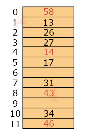
For example, let the hash function be h(k) = k mod 12 and let the keys be 31, 26, 43, 27, 34, 46, 14, 58, 13, 17, 22. Then,
h(31) = 7
h(26) = 2
h(43) = 7
h(27) = 3
h(34) = 10
h(46) = 10
h(14) = 2
h(58) = 10
h(13) = 1
h(17) = 5
Thus, the collision occurs at 43, 46, 14, 58, 22.
Therefore, H(43, 1) = [h(43) + 1] mod 12 = 8mod12 = 8
H(46, 1) = [h(46)+1]mod12 = 11mod12 = 11
H(14, 1) = [h(14)+1]mod12 = 3mod12 = 3
But, index 3 is already filled, therefore, we will solve this for i=2.
H(14, 2) = h(14)+2 mod12 = 4
H(58, 1) = [h(58)+1]mod12 = 11
But 11th index already has a value, so perform hashing for i=2
H(58, 2) = [h(58)+2]mod12 = 0
Next, h(22) has a collision. But slots of index 10, 11, 0, 1, 2, 3, 4, 5 are already filled. This is a primary cluster.
In order to find a free slot, we need to get through this group of clusters. This increases the number of comparisons. In the worst case, the number of comparisons could be m-1 where m = size of the hash table.
To resolve this problem, quadratic probing was introduced.
2. Quadratic Probing:
In quadratic probing, the degree of i is 2 where i is the collision number. Thus, in quadratic probing, the hash function formed is:
H(k, i) = [h(k) + i2] mod m
However, quadratic probing has a drawback. There are chances of secondary clustering in quadratic probing.
Secondary clustering:
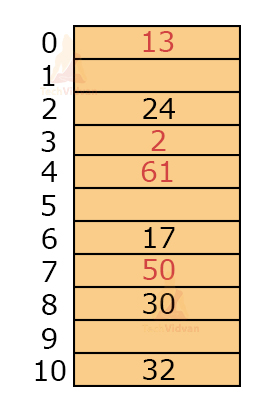
Let us understand the concept of secondary clustering with the help of an example.
Let keys = 24, 17, 32, 2, 13, 50, 30, 16 and let m = 11 for h(k) = k mod m.
Then,
h(24) = 2
h(17) = 6
h(32) = 10
h(2) = 2
h(13) = 2
h(50) = 6
h(30) = 8
h(61) = 6
Here, 3 keys are mapping to the same location: 24, 2, 13. Suppose the 2nd index is already filled, then a collision occurs for all three keys.
To find the next possible value, we will compute H(k) as follows:
H(24, 1) = 3
H(2, 1) = 3
H(13, 1) = 3
If 3rd index is already filled, then we will look for the next possible value.
H(24, 2) = 6
H(2, 2) = 6
H(13, 2) = 6
Similarly, if we check for consequent values, they will produce the same index.
From here, we can conclude that the keys that are mapped to the same memory location follow the same collision resolution path. In this example, the number of free slots is 5 and the number of filled slots are 6. But, every time we are reaching those 6 filled slots. Due to this, we can’t utilize the table effectively, as we can’t reach those free slots.
3. Double Hashing:
As the name suggests, in double hashing, we use two hash functions instead of one. If a collision occurs due to one hash function we can make use of the other hash function to find the next free slot.
Let H(k) represent the new hash function formed. Then, its value will be:
H(k, i) = [h(k) + i* h’(k)] mod m
Here, h(k) = primary hash function
And, h’(k) = secondary hash function
Separate Chaining:
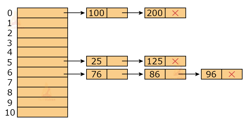
In separate chaining, we store all the values with the same index with the help of a linked list. This technique functions by maintaining a list of nodes.
For example, let the keys be 100, 200, 25, 125, 76, 86, 96 and let m = 10. Given, h(k) = k mod 10
Then, h(100) = 100 mod 10 = 0
h(200) = 200 mod 10 = 0
h(25) = 25 mod 10 = 5
h(125) = 125 mod 10 = 5
h(76) = 76 mod 10 = 6
h(86) = 86 mod 10 = 6
h(96) = 96 mod 10 = 6
Then, the values will be as follows and the linked list will be maintained.
Drawback of Separate chaining: The use of a linked list requires extra pointers. For n keys, there will be n extra pointers. If the table size is m, then the number of pointers will be (m+n).
Implementation of hash table in C:
#include <stdio.h>
#include <stdlib.h>

struct set
{
    int key;
    int value;
};
struct set *array;
int capacity = 10;
int size = 0;

int Hash_function(int key)
{
    return (key % capacity);
}

int check_prime(int n)
{
    int i;
    if (n == 1 || n == 0)
        return 0;
    for (i = 2; i < n / 2; i++)
    {
        if (n % i == 0)
            return 0;
    }
    return 1;
}

int get_prime(int n)
{
    if (n % 2 == 0)
        n++;
    while (!check_prime(n))
        n += 2;
    return n;
}

void init_array()
{
    capacity = get_prime(capacity);
    array = (struct set *)malloc(capacity * sizeof(struct set));
    for (int i = 0; i < capacity; i++)
    {
        array[i].key = 0;
        array[i].value = 0;
    }
}

void insert(int key, int value)
{
    int index = Hash_function(key);
    if (array[index].value == 0)
    {
        array[index].key = key;
        array[index].value = value;
        size++;
        printf("\n Key (%d) has been inserted \n", key);
    }
    else if (array[index].key == key)
        array[index].value = value;
    else
        printf("\n Collision occured  \n");
}

void Remove_element(int key)
{
    int index = Hash_function(key);
    if (array[index].value == 0)
        printf("\n This key does not exist \n");
    else
    {
        array[index].key = 0;
        array[index].value = 0;
        size--;
        printf("\n Key (%d) has been removed \n", key);
    }
}

void display()
{
    int i;
    for (i = 0; i < capacity; i++)
    {
        if (array[i].value == 0)
            printf("\n array[%d]: / ", i);
         else
            printf("\n key: %d array[%d]: %d \t", array[i].key, i, array[i].value);
    }
}

int size_of_hashtable()
{
    return size;
}

int main()
{
    int choice, key, value, n;
    int c = 0;
    init_array();

    do
    {
        printf("1.Insert item in the Hash Table"
        "\n2.Remove item from the Hash Table"
        "\n3.Check the size of Hash Table"
        "\n4.Display a Hash Table"
        "\n\n Please enter your choice: ");

        scanf("%d", &choice);
        switch (choice)
        {
            case 1:
                printf("Enter key -:\t");
                scanf("%d", &key);
                printf("Enter data -:\t");
                scanf("%d", &value);
                insert(key, value);
                break;

            case 2:
                printf("Enter the key to delete-:");
                scanf("%d", &key);
                Remove_element(key);
                break;

            case 3:
                n = size_of_hashtable();
                printf("Size of Hash Table is-:%d\n", n);
                break;

            case 4:
                display();
                break;

            default:
                printf("Invalid Input\n");
        }

        printf("\nDo you want to continue (press 1 for yes): ");
        scanf("%d", &c);

    } while (c == 1);
}
Hash Table Implementation in C++:
#include <bits/stdc++.h>

struct set
{
    int key;
    int value;
};
struct set *array;
int capacity = 10;
int size = 0;

int Hash_function(int key)
{
    return (key % capacity);
}

int check_prime(int n)
{
    int i;
    if (n == 1 || n == 0)
        return 0;
    for (i = 2; i < n / 2; i++)
    {
        if (n % i == 0)
            return 0;
    }
    return 1;
}

int get_prime(int n)
{
    if (n % 2 == 0)
        n++;
    while (!check_prime(n))
        n += 2;
    return n;
}

void init_array()
{
    capacity = get_prime(capacity);
    array = (struct set *)malloc(capacity * sizeof(struct set));
    for (int i = 0; i < capacity; i++)
    {
        array[i].key = 0;
        array[i].value = 0;
    }
}

void insert(int key, int value)
{
    int index = Hash_function(key);
    if (array[index].value == 0)
    {
        array[index].key = key;
        array[index].value = value;
        size++;
        cout << "\n Key (%d) has been inserted \n"<< key;
    }
    else if (array[index].key == key)
        array[index].value = value;
    else
        cout <<"\n Collision occured  \n";
}

void Remove_element(int key)
{
    int index = Hash_function(key);
    if (array[index].value == 0)
        cout << "\n This key does not exist \n";
    else
    {
        array[index].key = 0;
        array[index].value = 0;
        size--;
        cout << "\n Key (%d) has been removed \n" << key;
    }
}

void display()
{
    int i;
    for (i = 0; i < capacity; i++)
    {
        if (array[i].value == 0)
            cout <<"\n array[%d]: / " << i;
         else
            cout <<"\n key: %d array[%d]: %d \t"<< array[i].key << i << array[i].value;
    }
}

int size_of_hashtable()
{
    return size;
}

int main()
{
    int choice, key, value, n;
    int c = 0;
    init_array();

    do
    {
        cout <<"1.Insert item in the Hash Table"
        "\n2.Remove item from the Hash Table"
        "\n3.Check the size of Hash Table"
        "\n4.Display a Hash Table"
        "\n\n Please enter your choice: ";

        cin >> choice;
        switch (choice)
        {
            case 1:
                cout <<"Enter key -:\t";
                cin >> key;
                printf(cout <<"Enter data -:\t";
                cin >> value;
                insert(key, value);
                break;

            case 2:
                cout << "Enter the key to delete: ";
                cin >> key;
                Remove_element(key);
                break;

            case 3:
                n = size_of_hashtable();
                cout << "Size of Hash Table is-:%d\n" << n;
                break;

            case 4:
                display();
                break;

            default:
                cout << "Invalid Input\n";
        }

        cout << "\nDo you want to continue (press 1 for yes): ";
        cin >> c;

    } while (c == 1);
}
Implementation of hash table in Java:
import java.util.*;

class Hash_Table {
  public static void main(String args[])
  {
  hash_table<Integer, Integer>
    ht = new hash_table<Integer, Integer>();

  ht.put(123, 432);
  ht.put(12, 2345);
  ht.put(15, 5643);
  ht.put(3, 321);

  ht.remove(12);

  System.out.println(ht);
  }
}
Implementation of hash Function in Python:
hash_table = [[],] * 10

def check_prime(n):
    if n == 1 or n == 0:
        return 0

    for i in range(2, n//2):
        if n % i == 0:
            return 0
    return 1


def get_prime(n):
    if n % 2 == 0:
        n = n + 1

    while not check_prime(n):
        n += 2
    return n


def hash_function(key):
    capacity = get_prime(10)
    return key % capacity


def insert_value(key, value):
    index = hash_function(key)
    hash_table[index] = [key, value]

def remove_value(key):
    index = hash_function(key)
    hash_table[index] = 0

insert_value(123, "C")
insert_value(432, "DS")
insert_value(213, "Python")
insert_value(654, "Java")

print(hash_table)

remove_value(123)

print(hash_table)
Applications of Hashing:
- In Symbol table
- For constant-time lookup operations and insertion operations
- In Domain name Servers(DNS)
- In cryptography applications
Conclusion:
Hashing is a very good technique to reduce or solve the computational problems in O(1) time. However, we need to note that, hashing does produce results in O(1) time. Whenever collisions occur, the time complexity increases. Thus, the best way to make use of hashing techniques and hash tables is by avoiding collisions.

